![\includegraphics[width=15cm]{rprojectsingle.eps}](img1544.png) A dendrogram
of a
single-link clustering of 30 documents from Reuters-RCV1.
Two possible cuts of the dendrogram are shown: at 0.4 into 24
clusters and at 0.1 into 12 clusters.
A dendrogram
of a
single-link clustering of 30 documents from Reuters-RCV1.
Two possible cuts of the dendrogram are shown: at 0.4 into 24
clusters and at 0.1 into 12 clusters.
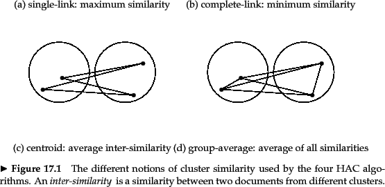
Before looking at specific similarity measures used in HAC in Sections 17.2 -17.4 , we first introduce a method for depicting hierarchical clusterings graphically, discuss a few key properties of HACs and present a simple algorithm for computing an HAC.
An HAC clustering is typically
visualized as a dendrogram as shown in
Figure 17.1 . Each merge is represented by a horizontal line.
The y-coordinate of the horizontal line is the
similarity of the two clusters that were
merged,
where documents are viewed as singleton clusters.
We call this similarity
the
combination similarity of the merged cluster.
For example, the combination similarity
of the cluster consisting of Lloyd's CEO questioned and
Lloyd's chief / U.S. grilling in Figure 17.1 is ![]() .
We define the combination similarity of a
singleton cluster as its document's self-similarity
(which is 1.0 for cosine similarity).
.
We define the combination similarity of a
singleton cluster as its document's self-similarity
(which is 1.0 for cosine similarity).
By moving up from the bottom layer to the top node, a dendrogram allows us to reconstruct the history of merges that resulted in the depicted clustering. For example, we see that the two documents entitled War hero Colin Powell were merged first in Figure 17.1 and that the last merge added Ag trade reform to a cluster consisting of the other 29 documents.
A fundamental assumption in HAC is that the merge operation
is monotonic . Monotonic means that if
![]() are the combination
similarities of the successive merges of an HAC, then
are the combination
similarities of the successive merges of an HAC, then
![]() holds. A non-monotonic hierarchical clustering
contains at least one inversion
holds. A non-monotonic hierarchical clustering
contains at least one inversion ![]() and
contradicts the fundamental assumption that we
and
contradicts the fundamental assumption that we
chose the best merge available at each step. We will see an example of an inversion in Figure 17.12 .
Hierarchical clustering does not require a prespecified number of clusters. However, in some applications we want a partition of disjoint clusters just as in flat clustering. In those cases, the hierarchy needs to be cut at some point. A number of criteria can be used to determine the cutting point:
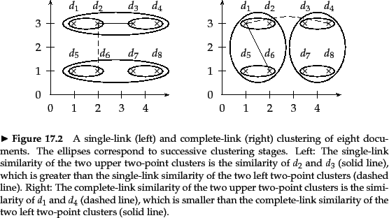
A simple, naive HAC algorithm is shown in
Figure 17.2 .
We first compute the
![]() similarity matrix
similarity matrix ![]() .
The algorithm then executes
.
The algorithm then executes
![]() steps of merging the currently most
similar clusters.
In each iteration,
the two most similar clusters are merged and the rows and columns of the
merged cluster
steps of merging the currently most
similar clusters.
In each iteration,
the two most similar clusters are merged and the rows and columns of the
merged cluster ![]() in
in ![]() are updated.
are updated.![]() The clustering is stored as a list of merges in
The clustering is stored as a list of merges in ![]() .
.
![]() indicates which clusters are still available to be
merged. The function
SIM
indicates which clusters are still available to be
merged. The function
SIM![]() computes the similarity of cluster
computes the similarity of cluster ![]() with
the merge of clusters
with
the merge of clusters ![]() and
and ![]() . For some HAC algorithms,
SIM
. For some HAC algorithms,
SIM![]() is simply a function of
is simply a function of ![]() and
and
![]() , for example,
the maximum of these two values for single-link.
, for example,
the maximum of these two values for single-link.
We will now refine this algorithm for the different similarity measures of single-link and complete-link clustering (Section 17.2 ) and group-average and centroid clustering ( and 17.4 ). The merge criteria of these four variants of HAC are shown in Figure 17.3 .