Mutual information

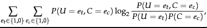
A common feature selection method is to compute $A(\tcword,c)$ as the expected mutual information (MI) of term $\tcword$ and class $c$. MI measures how much information the presence/absence of a term contributes to making the correct classification decision on $c$. Formally:

$$I(\wvar;C) = \sum_{e_\tcword \in \{ 1,0 \} } \sum_{e_c \in \{ 1,0 \} } P(\wvar... ...rd,C=e_c) \log_2 \frac {P(\wvar=e_\tcword,C=e_c)} {P(\wvar=e_\tcword)P(C=e_c)},$$ (130)

where $\wvar$ is a random variable that takes values $e_\tcword=1$ (the document contains term $\tcword$) and $e_\tcword=0$ (the document does not contain $\tcword$), as defined on page 13.4 , and $C$ is a random variable that takes values $e_c=1$ (the document is in class $c$) and $e_c=0$ (the document is not in class $c$). We write $\wvar_\tcword$ and $C_c$ if it is not clear from context which term $\tcword$ and class $c$ we are referring to.

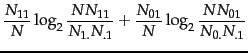
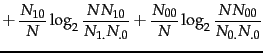
For MLEs of the probabilities, Equation 130 is equivalent to Equation 131:

$$I(\wvar;C) = \frac{\observationo_{11}}{N}\log_2 \frac{N \observationo_{11}}{\o... ...01}}{N}\log_2 \frac{N \observationo_{01}}{\observationo_{0.}\observationo_{.1}}$$ (131)

$$+\, \frac{\observationo_{10}}{N}\log_2 \frac{N \observationo_{10}... ...00}}{N}\log_2 \frac{N \observationo_{00}}{\observationo_{0.}\observationo_{.0}}$$ (132)

where the $\observationo$s are counts of documents that have the values of $e_\tcword$ and $e_c$ that are indicated by the two subscripts. For example, $\observationo_{10}$ is the number of documents that contain $\tcword$ ($e_\tcword=1$) and are not in $c$ ($e_c=0$). $\observationo_{1.} = \observationo_{10}+\observationo_{11}$ is the number of documents that contain $\tcword$ ($e_\tcword=1$) and we count documents independent of class membership ( $e_c \in \{ 0, 1\}$). $N=\observationo_{00}+\observationo_{01}+\observationo_{10}+\observationo_{11}$ is the total number of documents. An example of one of the MLE estimates that transform Equation 130 into Equation 131 is $P(\wvar=1,C=1)=\observationo_{11}/N$.

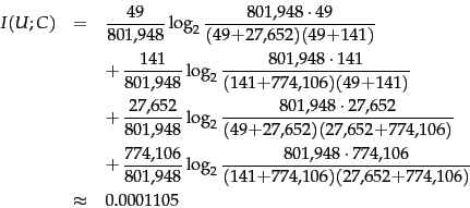
Worked example. Consider the class poultry and the term export in Reuters-RCV1. The counts of the number of documents with the four possible combinations of indicator values are as follows:

	$e_c=e_{\class{poultry}}=1$	$e_c = e_{\class{poultry}}=0$
$e_\tcword=e_{\term{export}} = 1$	$\observationo_{11}=49$	$\observationo_{10} = 27{,}652$
$e_\tcword=e_{\term{export}} = 0$	$\observationo_{01} = 141$	$\observationo_{00}=774{,}106$

After plugging these values into Equation 131 we get:

$$\begin{eqnarray*} I(\wvar;C) &= &\frac{49}{801{,}948} \log_2\frac{ 801{,}948 \cd... ... \!774{,}106) (27{,}652\! + \!774{,}106)}\\ &\approx& 0.0001105 \end{eqnarray*}$$

End worked example.

To select $\ktopk$ terms $\tcword_1,\ldots,\tcword_\ktopk$ for a given class, we use the feature selection algorithm in Figure 13.6 : We compute the utility measure as $A(\tcword,c)=I(U_\tcword,C_c)$ and select the $\ktopk$ terms with the largest values.

Mutual information measures how much information - in the information-theoretic sense - a term contains about the class. If a term's distribution is the same in the class as it is in the collection as a whole, then $I(\wvar;C) = 0$. MI reaches its maximum value if the term is a perfect indicator for class membership, that is, if the term is present in a document if and only if the document is in the class.

Figure 13.7: Features with high mutual information scores for six Reuters-RCV1 classes.

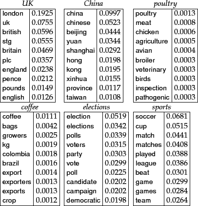Figure 13.7 shows terms with high mutual information scores for the six classes in Figure 13.1 . The selected terms (e.g., london, uk, british for the class UK) are of obvious utility for making classification decisions for their respective classes. At the bottom of the list for UK we find terms like peripherals and tonight (not shown in the figure) that are clearly not helpful in deciding whether the document is in the class. As you might expect, keeping the informative terms and eliminating the non-informative ones tends to reduce noise and improve the classifier's accuracy.

Figure 13.8: Effect of feature set size on accuracy for multinomial and Bernoulli models.

Such an accuracy increase can be observed in Figure 13.8 , which shows $F_1$ as a function of vocabulary size after feature selection for Reuters-RCV1. Comparing $F_1$ at 132,776 features (corresponding to selection of all features) and at 10-100 features, we see that MI feature selection increases $F_1$ by about 0.1 for the multinomial model and by more than 0.2 for the Bernoulli model. For the Bernoulli model, $F_1$ peaks early, at ten features selected. At that point, the Bernoulli model is better than the multinomial model. When basing a classification decision on only a few features, it is more robust to consider binary occurrence only. For the multinomial model (MI feature selection), the peak occurs later, at 100 features, and its effectiveness recovers somewhat at the end when we use all features. The reason is that the multinomial takes the number of occurrences into account in parameter estimation and classification and therefore better exploits a larger number of features than the Bernoulli model. Regardless of the differences between the two methods, using a carefully selected subset of the features results in better effectiveness than using all features.