Next: Relation to multinomial unigram
Up: Text classification and Naive
Previous: The text classification problem
Contents
Index
Naive Bayes text classification
The first supervised learning method
we introduce is the multinomial Naive Bayes
or
multinomial NB
model, a probabilistic learning method. The probability of a document  being in
class
being in
class  is computed as
 |
|
|
(113) |
where
 is the conditional probability of
term
is the conditional probability of
term
 occurring in a document of class
.
occurring in a document of class
.![[*]](http://nlp.stanford.edu/IR-book/html/icons/footnote.png) We interpret
as a measure of how much evidence
contributes that is the correct class.
We interpret
as a measure of how much evidence
contributes that is the correct class.
 is the prior probability of a document occurring in
class . If a document's terms do not provide clear
evidence for one class versus another, we choose the one that
has a higher prior probability.
is the prior probability of a document occurring in
class . If a document's terms do not provide clear
evidence for one class versus another, we choose the one that
has a higher prior probability.
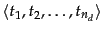 are the
tokens in that are part of the vocabulary we use for
classification and
are the
tokens in that are part of the vocabulary we use for
classification and  is the number of such tokens in . For example,
for the
one-sentence document Beijing and Taipei join
the WTO might be
is the number of such tokens in . For example,
for the
one-sentence document Beijing and Taipei join
the WTO might be
 , with
  , if
we treat the terms and and the as stop words.
, if
we treat the terms and and the as stop words.
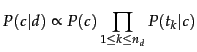
In text classification, our goal is to find the best
class for the document. The best class in NB classification
is the
most likely or
maximum a posteriori
( MAP ) class  :
:
 |
(114) |
We write  for
for  because we do not know the true
values of the parameters
because we do not know the true
values of the parameters
 and
and
 , but estimate them from the
training set as we will see in a moment.
, but estimate them from the
training set as we will see in a moment.
In Equation 114,
many conditional probabilities are
multiplied, one for each position
 .
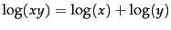
This can result in a floating point underflow. It
is therefore better to perform the computation by adding
logarithms of probabilities instead of multiplying
probabilities. The class with the highest log probability
score is still the most probable;
.
This can result in a floating point underflow. It
is therefore better to perform the computation by adding
logarithms of probabilities instead of multiplying
probabilities. The class with the highest log probability
score is still the most probable;
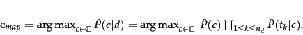
 and the logarithm function is monotonic. Hence,
the maximization that is actually done in most
implementations of NB is:
and the logarithm function is monotonic. Hence,
the maximization that is actually done in most
implementations of NB is:
![$\displaystyle c_{map} = \argmax_{\tcjclass \in \mathbb{C}} \ [ \log \hat{P}(\tc...
...{1 \leq \tcposindex \leq n_d}
\log \hat{P}(\tcword_\tcposindex\vert\tcjclass)].$](img882.png) |
|
|
(115) |
Equation 115 has a simple interpretation. Each
conditional parameter
 is a weight that
indicates how good an indicator
is for
is a weight that
indicates how good an indicator
is for
 . Similarly, the prior
 is a weight that indicates the relative frequency of
. More frequent classes are more likely to be the
correct class than infrequent
classes.
The
sum of log prior and term weights is then a measure of how
much evidence there is for the document being in the class, and
Equation 115 selects the class for which we have
the most evidence.
is a weight that indicates the relative frequency of
. More frequent classes are more likely to be the
correct class than infrequent
classes.
The
sum of log prior and term weights is then a measure of how
much evidence there is for the document being in the class, and
Equation 115 selects the class for which we have
the most evidence.
We will initially work with this intuitive interpretation of
the multinomial NB model and defer a formal derivation to
Section 13.4 .
How do we estimate the parameters
 and
and
 ?
We first try
the maximum likelihood estimate (MLE; probtheory), which
is simply the relative frequency and
corresponds to the most likely value of each parameter given
the training data. For the priors this estimate is:
?
We first try
the maximum likelihood estimate (MLE; probtheory), which
is simply the relative frequency and
corresponds to the most likely value of each parameter given
the training data. For the priors this estimate is:
 |
|
|
(116) |
where  is the number of documents in class and
 is the total number of documents.
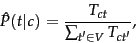
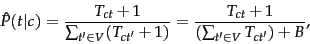
We estimate the conditional probability
 as the relative frequency
of term
as the relative frequency
of term  in
documents belonging to class :
in
documents belonging to class :
 |
(117) |
where  is the number of occurrences of in
training documents from class ,
including multiple
occurrences of a term in a document. We have made the
positional independence assumption here,
which we will discuss in more detail in the next section:
is a count of occurrences
in all positions
is the number of occurrences of in
training documents from class ,
including multiple
occurrences of a term in a document. We have made the
positional independence assumption here,
which we will discuss in more detail in the next section:
is a count of occurrences
in all positions  in the documents in the training set.
Thus, we do not compute different estimates for different
positions and, for example, if a word occurs twice in a document, in positions
in the documents in the training set.
Thus, we do not compute different estimates for different
positions and, for example, if a word occurs twice in a document, in positions
 and
and  , then
 .
.
The problem with the MLE estimate is that it is zero for a
term-class combination that did not occur in the training
data. If
the term WTO in the training data only
occurred in China documents, then the MLE estimates
for the other classes, for example UK, will be
zero:
 |
(118) |
Now, the one-sentence document Britain is a
member of the WTO
will get a conditional probability of
zero for UK because we are multiplying the conditional
probabilities for all terms in
Equation 113.
Clearly, the model should
assign a high probability to the UK class because
the term Britain
occurs. The problem is that the zero probability
for WTO cannot be ``conditioned away,'' no
matter how strong the evidence for the class UK
from other features.
The estimate is 0 because of
sparseness : The training data are never large enough
to represent the frequency of rare events adequately, for
example,
the frequency of WTO occurring in
UK documents.
Figure 13.2:
Naive Bayes algorithm (multinomial model):
Training and testing.
![\begin{figure}\begin{algorithm}{TrainMultinomialNB}{\mathbb{C},\docsetlabeled}
V...
...OR}\\
\RETURN{\argmax_{c \in \mathbb{C}} score[c]}
\end{algorithm}
\end{figure}](img897.png) |
To eliminate zeros, we use
add-one
or Laplace
smoothing, which simply
adds one to each count (cf. Section 11.3.2 ):
 |
(119) |
where  is the number of terms in the vocabulary.
Add-one smoothing
can be interpreted as a uniform prior (each term occurs once
for each class) that is then updated as evidence
from the training data comes in. Note that this is
a prior probability for the occurrence of a term as opposed
to the prior probability of a class which we estimate in
Equation 116 on the document level.
is the number of terms in the vocabulary.
Add-one smoothing
can be interpreted as a uniform prior (each term occurs once
for each class) that is then updated as evidence
from the training data comes in. Note that this is
a prior probability for the occurrence of a term as opposed
to the prior probability of a class which we estimate in
Equation 116 on the document level.
We have now introduced all the elements we need for training
and applying an NB classifier. The complete
algorithm is described in
Figure 13.2 .
Table 13.1:
Data for parameter
estimation examples.
| | |
docID |
words in document |
in  China? China? |
|
| | training set |
1 |
Chinese Beijing Chinese |
yes |
|
| | |
2 |
Chinese Chinese Shanghai |
yes |
|
| | |
3 |
Chinese Macao |
yes |
|
| | |
4 |
Tokyo Japan Chinese |
no |
|
| | test set |
5 |
Chinese Chinese Chinese Tokyo Japan |
? |
|
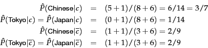
Worked example.
For the example in Table 13.1 , the multinomial
parameters we need to classify the test document are the
priors
 and
and
 and the
following conditional probabilities:
and the
following conditional probabilities:
The denominators are  and
and  because
the lengths of
because
the lengths of  and
and
 are
8 and 3, respectively, and because
the constant
are
8 and 3, respectively, and because
the constant  in
Equation 119 is 6 as the vocabulary consists of six
terms.
in
Equation 119 is 6 as the vocabulary consists of six
terms.
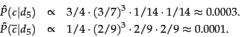
We then get:
Thus, the classifier assigns
the test document to = China. The reason for
this classification decision is that
the three occurrences of the positive
indicator Chinese in  outweigh the occurrences of
the two negative indicators Japan and Tokyo. End worked example.
outweigh the occurrences of
the two negative indicators Japan and Tokyo. End worked example.
Table 13.2:
Training and test times for
NB.
| | mode |
time complexity |
|
| | training |
 |
|
| | testing |
 |
|
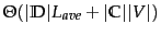
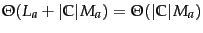
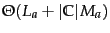
What is the time complexity of NB? The complexity
of computing the parameters is
 because
the set of parameters consists of
because
the set of parameters consists of
 conditional probabilities and
  priors. The
preprocessing necessary for computing the parameters
(extracting the vocabulary, counting terms, etc.) can be
done in one pass through the training data. The time
complexity of this component is therefore
priors. The
preprocessing necessary for computing the parameters
(extracting the vocabulary, counting terms, etc.) can be
done in one pass through the training data. The time
complexity of this component is therefore
 ,
where
,
where
 is the number of documents and
  is
the average length of a document.
is
the average length of a document.
We use
as a notation for  here, where
  is the length of the
training collection.
This is
nonstandard;
is the length of the
training collection.
This is
nonstandard;
 is not defined for an average.
We prefer expressing the time
complexity in terms of
is not defined for an average.
We prefer expressing the time
complexity in terms of
 and
because these are the primary statistics used to
characterize training collections.
and
because these are the primary statistics used to
characterize training collections.
The time complexity of
APPLYMULTINOMIALNB in
Figure 13.2 is
 .
.
 and
and  are the numbers of
tokens and types, respectively, in the test
document .
APPLYMULTINOMIALNB can be modified to be
are the numbers of
tokens and types, respectively, in the test
document .
APPLYMULTINOMIALNB can be modified to be
 (Exercise 13.6 ).
Finally, assuming
that the length of test documents is bounded,
because
(Exercise 13.6 ).
Finally, assuming
that the length of test documents is bounded,
because
 for a fixed constant
  .
.
Table 13.2 summarizes the time complexities.
In general, we have
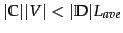 , so both training
and testing complexity are linear in the time it takes
to scan the data. Because we have to look at the data at
least once, NB can be said to have optimal time
complexity. Its efficiency is one reason why NB
is a popular text classification method.
, so both training
and testing complexity are linear in the time it takes
to scan the data. Because we have to look at the data at
least once, NB can be said to have optimal time
complexity. Its efficiency is one reason why NB
is a popular text classification method.
Subsections
Next: Relation to multinomial unigram
Up: Text classification and Naive
Previous: The text classification problem
Contents
Index
© 2008 Cambridge University Press
This is an automatically generated page. In case of formatting errors you may want to look at the PDF edition of the book.
2009-04-07