This is a cross-post from my personal blog.

We’ve finally published a neural network model which has been under development for over a year at Stanford. I’m proud to announce SPINN: the Stack-augmented Parser-Interpreter Neural Network. The project fits into what has long been the Stanford research program, mixing deep learning methods with principled approaches inspired by linguistics. It is the result of a substantial collaborative effort also involving Sam Bowman, Abhinav Rastogi, Raghav Gupta, and our advisors Christopher Manning and Christopher Potts.

This post is a brief introduction to the SPINN project from a particular angle, one which is likely of interest to researchers both inside and outside of the NLP world. I’ll focus here on the core SPINN theory and how it enables a hybrid tree-sequence architecture.¹ This architecture blends the otherwise separate paradigms of recursive and recurrent neural networks into a structure that is stronger than the sum of its parts.

(quick links: model description, full paper, code)

Our task, broadly stated, is to build a model which outputs compact, sufficient² representations of natural language. We will use these representations in downstream language applications that we care about.³ Concretely, for an input sentence \(\mathbf x\), we want to learn a powerful representation function \(f(\mathbf x)\) which maps to a vector-valued representation of the sentence. Since this is a deep learning project, \(f(\mathbf{x})\) is of course parameterized by a neural network of some sort.

Voices from Stanford have been suggesting for a long time that basic linguistic theory might help to solve this representation problem. Recursive neural networks, which combine simple grammatical analysis with the power of recurrent neural networks, were strongly supported here by Richard Socher, Chris Manning, and colleagues. SPINN has been developed in this same spirit of merging basic linguistic facts with powerful neural network tools.

Model

Our model is based on an insight into representation. Recursive neural networks are centered around tree structures (usually binary constituency trees) like the following:

In a standard recursive neural network implementation, we compute the representation of a sentence (equivalently, the root node S) as a recursive function of its two children, and so on down the tree. The recursive function is specified like this, for a parent representation \(\vec p\) with child representations \(\vec c_1, \vec c_2\): \[\vec p = \sigma(W [\vec c_1, \vec c_2])\] where \(\sigma\) is some nonlinearity such as the \(\tanh\) or sigmoid function. The obvious way to implement this recurrence is to visit each triple of a parent and two children, and compute the representations bottom-up. The graphic below demonstrates this computation order.

This is a nice idea, because it allows linguistic structure to guide computation. We are using our prior knowledge of sentence structure to simplify the work left to the deep learning model.

One substantial practical problem with this recursive neural network, however, is that it can’t easily be batched. Each input sentence has its own unique computation defined by its parse tree. At any given point, then, each example will want to compose triples in different memory locations. This is what gives recurrent neural networks a serious speed advantage. At each timestep, we merely feed a big batch of memories through a matrix multiplication. This work can be easily farmed out on a GPU, leading to order-of-magnitude speedups. Recursive neural networks unfortunately don’t work like this. We can’t retrieve a single batch of contiguous data at each timestep, since each example has different computation needs throughout the process.⁴

Shift-reduce parsing

The fix comes from the change in representation foreshadowed earlier. To make that change, I need to introduce a parsing formalism popular in natural language processing, originally stolen from the compiler/PL crowd.

Shift-reduce parsing is a method for building parse structures from sequence inputs in linear time. It works by exploiting an auxiliary stack structure, which stores partially-parsed subtrees, and a buffer, which stores input tokens which have yet to be parsed.

We use a shift-reduce parser to apply a sequence of transitions, moving items from the buffer to the stack and combining multiple stack elements into single elements. In the parser’s initial state, the stack is empty and the buffer contains the tokens of an input sentence. There are just two legal transitions in the parser transition sequence.

• Shift pulls the next token from the buffer and pushes it onto the stack.
• Reduce combines the top two elements of the stack into a single element, producing a new subtree. The top two elements of the stack become the left and right children of this new subtree.

The animation below shows how these two transitions can be used to construct the entire parse tree for our example sentence.⁵

Rather than running a standard bottom-up recursive computation, then, we can execute this table-based method on transition sequences. Here’s the buffer and accompanying transition sequence we used for the sentence above. S denotes a shift transition and R denotes a reduce transition.

Buffer: The, man, picked, the, vegetables
Transitions: S, S, R, S, S, S, R, R, R

Every binary tree has a unique corresponding shift-reduce transition sequence. For a sentence with \(n\) tokens, we can produce its parse with a shift-reduce parser in exactly \(2n - 1\) transitions.

All we need to do is build a shift-reduce parser that combines vector representations rather than subtrees. This system is a pretty simple extension of the original shift-reduce setup:

• Shift pulls the next word embedding from the buffer and pushes it onto the stack.
• Reduce combines the top two elements of the stack \(\vec c_1, \vec c_2\) into a single element \(\vec p\) via the standard recursive neural network feedforward: \(\vec p = \sigma(W [\vec c_1, \vec c_2])\).

Now we have a shift-reduce parser, deep-learning style.

This is really cool for several reasons. The first is that this shift-reduce recurrence computes the exact same function as the recursive neural network we formulated above. Rather than making the awkward bottom-up tree-structured computation, then, we can just run a recurrent neural network over these shift-reduce transition sequences.⁶

If we’re back in recurrent neural network land, that means we can make use of all the batching goodness that we were excited about earlier. It gains us quite a bit of speed, as the figure below from our paper demonstrates.

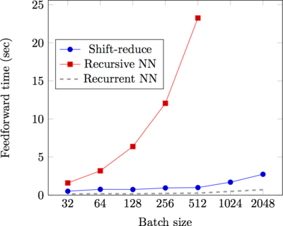
That’s up to a 25x improvement over our comparison recursive neural network implementation. We’re between two to five times slower than a recurrent neural network, and it’s worth discussing why. Though we are able to batch examples and run an efficient GPU implementation, this computation is fundamentally divergent — at any given timestep, some examples require a “shift” operation, and other examples require a “reduce.” When computing results for all examples in bulk, we’re fated to throw away at least half of our work.

I’m excited about this big speedup. Recursive neural networks have often been dissed as too slow and “not batchable,” and this development proves both points wrong. I hope it will make new research on this model class a practical opportunity.

Hybrid tree-sequence networks

I’ve been hinting throughout this post that our new shift-reduce feedforward is really just a recurrent neural network computation. To be clear, here’s the “sequence” that the recurrent neural network traverses when it reads in our example tree:

This is a post-order tree traversal, where for a given parent node we recurse through the left subtree, then the right, and then finally visit the parent.

We had a simple idea with a big result after looking at this diagram: why not have a recurrent neural network follow along this path of arrows?

Concretely, that means that at every timestep, we update some RNN memory regardless of the shift-reduce transition. We call this the tracking memory. We can write out the algorithm mathematically for clarity. At any given timestep \(t\), we compute a new tracking value \(\vec m_t\) by combining the top two elements of the stack \(\vec c_1, \vec c_2\), the top of the buffer \(\vec b_1\), and the previous tracking memory \(\vec m_{t-1}\): \begin{equation} \vec m_t = \text{Track}(\vec m_{t-1}, \vec c_1, \vec c_2, \vec b_1) \\ \end{equation} We can then pass this tracking memory onto the recursive composition function, via a simple extension like this: \begin{equation} \vec p = \sigma(W [\vec c_1; \vec c_2; \vec m_t]) \\ \end{equation} What have we done? We’ve just interwoven a recurrent neural network into a recursive neural network computation. The recurrent memories are used to augment the recursive computation (\(m_t\) is passed to the recursive composition function) and vice versa (the recurrent memories are a function of the recursively computed values on the stack).

We show in our paper how these two paradigms turn out to have complementary power on our test data. By combining the recurrent and recursive models into a single feedforward, we get a model that is more powerful than the sum of its parts.

What we’ve built is a new way to build a representation \(f(\mathbf x)\) for an input sentence \(\mathbf x\), like we discussed at the beginning of this post. In our paper, we use this representation to reach a high-accuracy result on the Stanford Natural Language Inference dataset.

This post managed to cover about one section of our full paper. If you’re interested in more details about how we implemented and applied this model, related work, or a more formal description of the algorithm discussed here, take a read. You can also check out our code repository, which has several implementations of the SPINN model and models which you can run to reproduce or extend our results.

We’re continuing active work on this project in order to learn better end-to-end models for natural language processing. I always enjoy hearing ideas from my readers — if this project interests you, get in touch via email or in the comment section below.

Acknowledgements

I have to first thank my collaborators, of course — this was a team of strong researchers with nicely complementary skills, and I look forward to pushing this further together with them in the future.

The SPINN project has been supported by a Google Faculty Research Award, the Stanford Data Science Initiative, and the National Science Foundation under grant numbers BCS 1456077 and IIS 1514268. Some of the Tesla K40s used for this research were donated to Stanford by the NVIDIA Corporation. Kelvin Gu, Noah Goodman, and many others in the Stanford NLP Group contributed helpful comments during development. Craig Quiter and Sam Bowman helped review this blog post.