Introduction

Our data were drawn from various categories or "topics" in the www.dmoz.org directory. This directory is similar in purpose and scope to Yahoo! and other web indices, although it is maintained by a community of volunteer editors, and unlike Yahoo! dmoz.org has an open licensing agreement that allows free use for derivative works, such as this research. Selecting documents that were pre-categorized guaranteed there was some underlying structure we could try to learn.

To evaluate our system’s performance, we carried along with each page its original category string under dmoz.org, such as "Sports/Badminton/". To measure the quality of the current learned clusters, we found, for each cluster, the most frequent original category string among its members (counting as members only items with a higher fractional expectation of being in this category than in any other). Then every member that matched this most frequent original category was counted as correctly categorized, and any other member was counted as an error.

This measure of accuracy had the advantage that achieving 100% percent meant we had exactly re-created the original clusters. It had the disadvantage that no "partial credit" was given for clustering similar documents together that happened to have been originally indexed separately, perhaps arbitrarily or mistakenly by a human editor. (We discovered at least once such mis-categorization, when a site on Chinese calligraphy ended up counting as an error in our calligraphy cluster, because it had been indexed under sculpture.)

It also gave no direct penalty to splitting an original single cluster into two or more parts, although such a split guaranteed that members of at least one other cluster would have to be counted as errors, since there would not be enough remaining clusters to go around.

Literature

We actually did very minimal literature review when starting this project, in part because of the very limited time for the project, and because we felt we would learn a great deal just "getting our hands dirty" with attempts to build and improve a clustering system.

We did take a close look at Hierarchically classifying documents using very few words, by Koller, D., Sahami, M., Proc. of the 14th International Conference on Machine Learning ICML97, pp. 170---178, 1997.

While this was a semi-supervised learning system, classifying computer science research papers into an existing hierarchical category tree, it did train Naïve Bayes classifiers using EM to let a large body of unlabeled training data improve the performance of the classifiers. It also used an extension to NB classifiers that learned limited dependencies among words, and learned a hierarchical set of classifiers, to reduce the size and scope of each classifier and improve reliability.

We also took a quick look at: A Corpus-Based Investigation of Definite Description Use, Massimo Poesio, Renata Vieira, Centre for Cognitive Science, The University of Edinburgh, and a few other papers on Kappa as an alternate measure of the reliability of our clusters. We decided that consistency of learned clusters from one run to the next was less meaningful than agreement with human editors, since learning such inane clusters as alphabetic ranges of the first word of the document would be completely consistent and repeatable, but equally useless as category clusters.

Design and Algorithms

The system we designed has two major parts: a Perl script for downloading, parsing, filtering, and caching the URLs as files of tokens, and a C++ program for reading and clustering the resulting files, and measuring the accuracy of the learned clusters.

We also chose to implement an optional stop-word list at this point, to remove high-frequency low-information common words. We started with a list of generally common English words, and supplemented it during development with vocabulary common to web pages, such as click, e-mail, visit, and site, with our final set including 156 words. Stop-word filtering, like most features of the script, could be controlled through command-line options, so comparative tests were simple to perform.

We also stripped out all characters other than letters, hyphens, apostrophes, and periods, and then dropped all tokens that contained no letters, or that were shorter than four characters. For almost all testing we shifted all text to lower-case, to better smooth the text distribution.

We eventually decided to parse the META tags for Keywords and Description, and include their text along with the page title in the cached file, each surrounded by delimiter tags so the cluster program could choose whether to include or even emphasize those words. This particularly helped classify some minimal pages that were the top of an HTML frame set or contained only a "splash" image. In keeping with the ever-changing structure of the Web, we discovered a fairly high fraction of pages listed in the dmoz.org directory were just "Click here for new location" pointers, or were frame sets or splash pages with no META tags or other significant text. A more sophisticated front end could try to recognize such pages and download the new location or child pages. We decided to simply discard pages that were shorter than 150 characters, once keywords, title, and description were included, which removed most of these unclassifiable pages from our test sets.

In our largest test set of 1493 URLs, 97% of the pages downloaded without an error, and of those, 75% passed the length threshold and were cached for clustering.

The initial version of our Perl front end would simply take a file of URLs and dmoz.org category strings, download, parse, and filter each one, and store it in a text file named after the original URL. It would also create an index file, containing all the filenames and category strings, which would serve as the initial input to the clustering stage. As we expanded our testing to cover larger and more challenging test sets, it became cumbersome to hand-construct the URL files. So we expanded the capabilities of our front end to be able to take a set of dmoz.org categories and create a URL file by reading the dmoz.org directory contents directly. Finally, in order to be able to create arbitrarily large test sets for scalability testing, we added the ability to randomly walk the dmoz.org directory and generate any number of "leaf node" categories.

We implemented various attempts at elimination "noise" words that were beyond what a fixed stop-word list could accomplish. An option (-r) would prune the word frequencies to remove all words that occurred in only one Document, since we considered learning single-document clusters to be outside our domain, and we learned that "outlier" pages could otherwise dominate some classifiers. Such words could obviously contribute no positive evidence in learning which documents to cluster together.

We also experimented with an option (-m N) to further prune the word frequencies to preserve only the N words in each document that occurred across the largest number of different documents. Any word in the entire vocabulary flagged to be thus preserved by any document was preserved in all documents, and all other words were deleted in every document.

Other options would delete words in each document that occurred £ N times (-f N), so –f 1 discarded singleton words, or would keep only the N most frequent types in each document (-k N). After all such pruning of word frequencies, they were renormalized.
 
 

We implemented K-means as "hard" clustering, in which each document belongs to only the closest cluster.

The halting condition is based on each document comparing its old vector of Expectations to the new one after each E-phase, finding the largest absolute change in the vector, and then finding the largest of these changes across all documents. If this maximum Expectation change is below some threshold (0.0001 for most of our testing), we conclude that EM has converged and halt.

We implemented two types of classifiers for use with the EM algorithm, with a command line option to select which one to use.

For each document’s expectations, it passed its word frequency map into the LogProb method of each cluster, and got back the Log Probability of that document "occurring," conditional on it being from that cluster. LogProb calculated the sum across every word in the document’s word frequency of the log of the product of that frequency and the classifier’s probability for that word. In probability space, this is the equivalent of computing the product across each word w in the document of P( w| c), which the Naïve Bayes assumption substitutes for the probability of the full document given the cluster, by assuming the individual words occur independently. This math is all done in Log space to avoid the risk of underflow from multiplying together many very small probabilities.

We calculate for each document D, for every cluster C:

where "norm" simply renormalizes each term as a probability by dividing by the sum of all terms across clusters. We chose to ignore the prior probability of each cluster P(C), assuming that every cluster was equally probable (i.e., of equal size). To calculate the exponent term, since the normalization needs to be done in Probability space, not Log space, we first subtracted from every LogProb the largest (most positive) LogProb value, then took the exponent of each term and normalized them. This subtraction was equivalent to multiplying each probability by the same (very large) constant value, which avoided underflow that would result from taking the exponent of such large negative numbers, and then disappeared when normalized.

This approach was really a "soft" variant of K-means clustering, permitting (and almost guaranteeing) fractional membership in multiple clusters, but using Euclidean distance for expectation weightings rather than a strictly probabilistic formula.

Results

Nonetheless, using EM with the cosine classifier gave us our only successful clustering behavior, and formed the basis for most of our further experiments and extensions.

K-means clustering never iterated more than once, because no document ever moved from the cluster to which it was initially (and randomly) assigned. Apparently, such "hard" clustering on the relatively small sets of data points (hundreds of documents), and the high dimensionality of the parameter space ( 10,000 words in the vocabulary), meant that any set of documents could find a centroid along some "word dimensions" that was closer than those any other sets.

Perhaps more surprisingly, the Naïve Bayes classifiers behaved quite similarly, in that documents rarely switched from the clusters to which they were first randomly assigned. We used various diagnostics to examine the causes, and discovered that almost every document contained words that were infrequent in other documents and therefore in other clusters. Since the membership of the document in its initial cluster guaranteed that every word in the document had a value in the classifier significantly greater than zero, it’s probability P(D|C) was significantly greater than zero in its cluster. But since every other cluster almost always had tiny epsilon smoothing values for one or more words in the document, the product of the probabilities across all words was nearly zero, even if many other words were a good match in frequency.

So the negative evidence of even one "missing" word in another cluster was enough to lock documents out of almost ever preferring a new cluster and switching.

We tried several variations in an attempt to "shake loose" this rigid stability of the NB clusters. We aggressively smoothed the expectation vectors (option –s), and thus the classifier distributions, by adding 1.0 to each expectation in the document and renormalizing. This was equivalent to setting each expectation E to (E+1)/(N+1), where N is the number of clusters, or an interpolation of each E with 1/N. The result was that expectations started and remained more evenly spread across the clusters, but a cluster that started with a slight lead over the others for a document, tended strongly to maintain that lead. Expectations tended to converge quickly to 2/(N+1) for the initial cluster and 1/(N+1) for the others. This was again due to the power with NB classifiers of negative evidence, even though this was somewhat weakened by every cluster having a significant fraction of each document’s word frequencies.

Another variation was in initialization of expectations before the first M-phase (-i option). Rather than assign each document entirely to a single cluster (except for the epsilon smoothing), each expectation was set to 1/N, and then slightly randomly perturbed by up to 1%. This too had little effect on the pattern of rigid convergence to the initially leading clusters, even when combined with the aggressive smoothing option.

Fortunately, the behavior of the "soft" cosine was much more promising. On our simplest test set of 22 documents from only 2 categories, the base cosine measure, with no additional options, achieved 100% accuracy on 20 out of 20 runs with different random starts. The random initial assignments had accuracies of between 54% and 72%. Throughout our tests with cosine, it always significantly improved accuracies over the random starting positions. While accuracies on the more complex test sets did vary with starting position, the best results were never due to the data already being "pre-clustered" by the random start.

When we ran the system on our next most difficult test set, "Set2" consisting of 73 URLs drawn from 5 widely-spaced different dmoz.org categories, we began seeing more complex patterns of convergence. In particular, the accuracy would always peak in accuracy and decline, usually within 5 iterations, at an average of 84% correct, but then continue iterating another 60+ times before the Expectation deltas converged, with a final accuracy averaging below 69%.

Clearly what EM was minimizing in its gradient descent, the differences between the cluster centroids and the fractional document expectations, did not map precisely to minimizing deviation from the original human-generated category labels. These two were clearly related, however, in that EM consistently reached a much-improved level of accuracy before overshooting on its way down its error slope.

At this point we implemented and tested several of the options described above, including pruning out words on various criteria, and options to emphasize words in the title (-e N) or in META tag keywords (-y N), counting such words as though they occurred N times instead of just once.

We discovered that the cruder methods for removing infrequent "noise" words substantially reduced accuracy. When we examined some basic word counts across the cached text files, we discovered that infrequent words often contained critical information about the topic of the page. For example within a Badminton category, of the 12 documents that contained the word "badminton," 4 of them used it only once, so stripping out singletons within documents, or keeping only the N most frequent words, discarded important information more than it filtered out irrelevant noise.

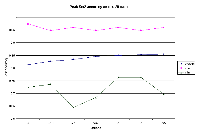
Since peak accuracy seemed to vary widely from run to run, even with the same options, we realized we needed to perform multiple runs to reduce the stochastic noise in our accuracy measurements. We used a set of simple scripts to let us run batches of 20 runs with a particular set of options, store the results, and filter out the significant numbers. Among the options that did not severely reduce peak accuracy (see Figure 1), there was disappointingly little variance from the base (no options) system. Since there is still some stochastic noise from random starting conditions in this data, even averaged over 20 runs, differences of 1 or 2% in accuracy could easily be due to chance, rather than a true difference in performance. Emphasizing title words slightly hurt performance, probably due to the many non-descriptive titles such as "Anne’s Corner of the Web." Emphasizing keywords by 5 seemed to help a bit, although tests on other sets would should such emphasis having a negative effect.

We also experimented briefly with trying to "guess" where the peak accuracy would occur, so we could halt EM iterations at that point. We noticed that, even across test sets, there was a consistent "elbow" in the curve of declining expectation deltas around the point of maximum accuracy. So we constructed a measure of the second derivative of Expectations that could usually predict within one or two iterations where a good halting point would be.

We also noticed a pattern that one or two clusters tended to go "extinct" in most runs. While they still could contain some fractional expectation of some documents, no document had them as their highest-expectation cluster when EM converged, and so they contributed nothing to the final accuracy score.

Clearly though, a different approach was needed to significantly improve system performance, and to more robustly deal with the disconnect between peak accuracy and convergence.

Enhancements

To accomplish this, we added an entropy option (-h K) that would keep in each classifier, in each M-phase iteration, only the K words with the lowest entropy for distinguishing documents being inside the cluster vs. outside. Besides calculating the normalized classifier as the expectation-weighted average of member documents’ word frequencies, we also constructed an "anti-classifier" for each cluster, of the average weighted distribution of words across all the other clusters. We could then examine each pair of frequencies of each word, and calculate the entropy using the following formula. We developed this ourselves, having not found an equation for information gain based on fractional data samples, with the counts of data instances (documents) all normalized away.

For each word type w, let f_w be the frequency with which it occurs in the current cluster, and f_w’ be its frequency across all other clusters. Then the probability of being in this cluster given that the word occurs is Pcw+ = f_w / (f_w + f_w’ ) and the probability of being in a different cluster given the word occurs in 1 – Pcw+. The probability of being in this cluster given the word doesn’t occur is Pcw– = (1 – f_w ) / ((1 – f_w ) + (1 – f_w’ )) of being in a different cluster, 1 – Pcw–. Also the overall probability of the word occurring, assuming N equal–sized clusters, is the weighted sum of f_w and f_w’,
Pw = (f_w / N) + f_w’ ´ (N – 1) / N. Then the entropy of cluster membership given the word occurred is
Hw = – (Pcw+ ´ log Pcw+) – ((1 – Pcw+) ´ log (1 – Pcw+)) bits. And the corresponding entropy given the word not occurring is Hw’ = – (Pcw– ´ log Pcw–) – ((1 – Pcw–) ´ log (1 – Pcw–)) bits. And the total expected entropy from knowing whether this word occurred is the weighted sum of these two values:

Htotal = Hw ´ Pw + Hw’ ´ (1 – Pw).

Testing with a pair of artificial documents with only a handful of words confirmed that Htotal has the desired behavior that it is 1 (no information gain) for words with equal distribution in and out of the cluster, and it’s lowest for words that occur only in one distribution but not the other. And for different word pairs with the same ratio of frequency, it’s lower for words with higher overall frequency (so the pair 0.04, 0.02 scores lower than the pair 0.02, 0.01).

The system builds a list of all the words in the classifier and their Htotal values, sorts it in ascending order, and removes all but the K lowest scoring words from the classifier. Although Htotal is symmetric whether the evidence of the word is positive or negative for membership in the cluster, (f_w > f_w’ or vice versa), our experience with Naïve Bayes classifiers led us to believe that the absence of a word was rarely a useful indicator. Only word pairs with f_w > f_w’ were considered when selecting the K best features.

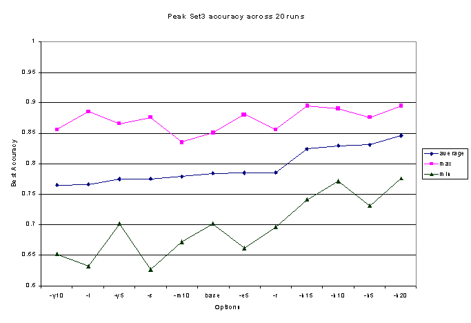
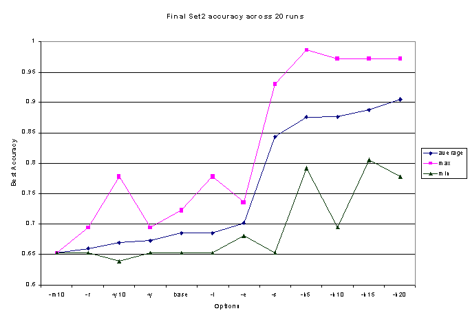
The improvements when testing on our larger more complex data sets were impressive. On Set3, containing 201 documents drawn from 7 more closely-related categories (3 under the visual arts, 2 under radio), the average peak accuracy jumped by 5% or more over any of the other enhancements we had attempted (See Figure 2). Just as importantly, using almost any value for –h K nearly eliminated problem with large declines in accuracy before convergence, and clusters going extinct. EM always converged at or within one or two documents of the highest accuracy achieved by any run using this feature selection (See Figure 3). And the rate of clusters going "extinct" fell dramatically as well, from 77% of runs on Set3 converging with 4 or more empty clusters (out of 7) to less than 6% of runs converging with a single empty cluster.

Also interestingly, our diagnostics displayed the words selected for each classifier after the final iteration (or in verbose mode, at every iteration), and these words often read like human-selected keywords for identifying that category. For instance, a Set3 "Radio Guides" cluster learned "radio, stations, live, world, music, audio, online, broadcasting, country, station, television, rock, and broadcast" as its highest-information words, and another on Calligraphy learned "calligraphy, lettering, hand, design, invitations, wedding, calligraphers, calligraphic, guild, calligrapher, join, gift, and weddings"

Both numerically and subjectively, this method of identifying relevant vs. irrelevant words was far superior to our other attempts.
 
 

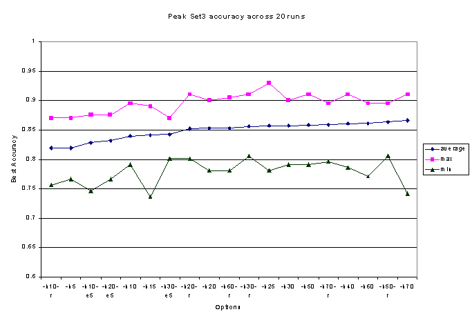
It did still have limitations, and our average accuracies across runs remained bounded at about 92% in Set2 and 87% for Set3 (see Figures 4). For Set2 the best accuracy was achieved with a relatively small set of K features, 10 or 20 words, while for Set3, accuracy continue to slightly increase up through 70 words, the largest we tested. This is probably due to the fact that the categories in Set2 are widely spaced, so few words are needed to distinguish between them, and a smaller set of higher-frequency words is less noisy and smoother. But with Set3’s closely-related categories, a much larger set of words is needed to simultaneously distinguish each cluster from both distant clusters and its nearby "siblings."

In examining the final clusters learned we also noted a problem when trying to learn clusters of very different sizes. The larger categories would often split their documents between 2 clusters, one of which would subsume a much smaller category, by including a few key words that identified those documents better than any other cluster. But most feature words were identical to the classifier for cluster with the other half of the documents from this category. The fractional expectations of many of these large-category documents was split almost evenly between these two clusters, while the subsumed smaller category documents generally had expectations close to 1 of being in their cluster together. Even when small clusters were successfully learned, it was clear from the fractional expectations of documents in large clusters, and the high-information feature words of the smaller clusters, that they had a large number of documents from the larger cluster with significant fractional membership in the small cluster. So even then a larger cluster was close to dividing and subsuming the small cluster.
 
 

We ran out of time to really analyze and address this limitation. One possible approach would be to somehow discount "minority" fractional members of a cluster in favor of members with a very high expectation of membership, in particular when the number of fractional members is very large compared to the high expectation members. Another would be to examine our assumptions our expected entropy calculations about equal-sized clusters, and consider removing or weakening any current bias towards learning clusters of roughly equal size.

Unfortunately, our algorithm for computing information gain for feature selection would need considerable redesign to be able to run faster than O(N²DV), so each iteration would take upwards of 8 hours on this largest set. We scaled back the set size to 48 clusters and 454 documents, and a single run using the –h 50 option reached an accuracy of 68% in 13 iterations then slowly declined to 65% over another 90 iterations, when we terminated it after 14 hours. Clearly substantial redesign and testing would be needed before this approach could successfully cluster any large portion of the full dmoz.org directory, if then.

Conclusions

We achieved a fairly high level of agreement with human editors in clustering moderately-sized sets of web pages, even when topics were closely related. Examining some of the mis-classified pages on our better test runs showed that many of them were probably unclassifiable based on only their content text, being longer-than usual "we’ve moved" pages, "choose hi/lo BW" or other splash pages. And a few were extreme outliers in word frequency for their category, such as a Palm Pilot page that never used words like palm, pilot, handheld, or software.

The improvements from information gain feature selection were impressive, particularly considering our fairly casual understanding of the theory behind it. A more complex application of information theory might be the best way to address the remaining problems of large clusters consuming smaller ones, clusters going empty.

The scalability of this approach remains a major weakness, and it might never scale to domains of hundreds of categories or more, even with further analysis and optimization. But it does seem to indicate that a simple text frequency analysis contains extremely relevant information about the topical similarity of pages. Such clustering might be a reasonable first stage when creating an index of smaller sets of documents, such as the pages within a company or departmental web site.