Tom Griffiths
gruffydd@psych.stanford.edu
Estimation of sparse multinomial distributions is an important component of many statistical learning tasks, and is particularly relevant to natural language processing. From their origins in [#!shannon51!#], statistical approaches to natural language typically require knowledge of the probability of a symbol or word conditioned upon some context. These probabilities are usually estimated from limited data, and require some form of smoothing before they can be used in a particular task. Consequently, a number of approaches to smoothing multinomial distributions have been suggested, typically combining statistical notions with heuristic strategies [#!cheng98!#]. In this paper, I present a generalization of a probabilistically correct approach to parameter estimation for sparse multinomial distributions. This new approach takes advantage of specific knowledge that we might have about a particular domain, such as natural language.
Perhaps the simplest and most elegant method of estimating a multinomial
distribution is a generalization of an approach originally taken by
Laplace. In the following discussion, I follow the presentation in
[#!friedmans98!#]. For a language ![]() containing
containing ![]() distinct
symbols, a multinomial distribution is specified by a parameter vector
distinct
symbols, a multinomial distribution is specified by a parameter vector
![]() , where
, where
![]() is the probability of an observation being symbol
is the probability of an observation being symbol ![]() .
Consequently, we have the constraints that
.
Consequently, we have the constraints that
![]() and
and
![]() . The task of multinomial estimation
is to take a data set
. The task of multinomial estimation
is to take a data set ![]() and produce a vector
and produce a vector ![]() that
results in a good approximation to the distribution that produced
that
results in a good approximation to the distribution that produced ![]() .
In this case, a data set
.
In this case, a data set ![]() consists of
consists of ![]() independent observations
independent observations
![]() drawn from the distribution to be estimated, which can be
summarised by the statistics
drawn from the distribution to be estimated, which can be
summarised by the statistics ![]() specifying the number of times the
specifying the number of times the
![]() th symbol occurs in the data.
th symbol occurs in the data. ![]() also specifies the set
also specifies the set ![]() of symbols that occur at least once in the training data.
of symbols that occur at least once in the training data.
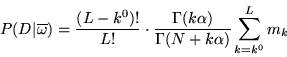
Stated in this way, the task of multinomial estimation can be framed as
one of predicting the next observation based on the data. Specifically,
we wish to calculate ![]() . The Bayesian estimate for this
probability is given by
. The Bayesian estimate for this
probability is given by
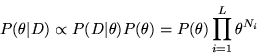
The above approach to estimating the parameters of a multinomial
distribution was first exploited by Laplace [#!laplace95!#], who took a
uniform prior
over ![]() to give the famous ``law of succession'':
to give the famous ``law of succession'':
![]() . A more general approach is to
assume a Dirichlet prior over
. A more general approach is to
assume a Dirichlet prior over ![]() , which is conjugate to the
multinomial distribution and gives
, which is conjugate to the
multinomial distribution and gives
The simple Bayesian method outlined above is appropriate for the general
task of multinomial estimation, but generally provides poor results when
used for smoothing of sparse multinomial distributions. This is
primarily a consequence of the erroneous assumption that all ![]() categories should be considered as possible values for
categories should be considered as possible values for ![]() . In
actuality, sparse multinomial distributions are characterized by the
fact that only a few symbols actually occur. In such cases, applying the
above method will give too much probability to symbols that never occur
and consequently give a poor estimate of the true distribution.
. In
actuality, sparse multinomial distributions are characterized by the
fact that only a few symbols actually occur. In such cases, applying the
above method will give too much probability to symbols that never occur
and consequently give a poor estimate of the true distribution.
In order to extend the Bayesian approach to sparse multinomial
distributions, several authors have used the notion of maintaining
uncertainty over the vocabulary from which observations are produced as
well as their probabilities. In [#!ristad95!#], Ristad uses assumptions
about the probability of strings based upon different vocabularies to give
the estimate
A more explicitly Bayesian approach is taken by Friedman and Singer in
[#!friedmans98!#], who also point out that Ristad's method can be
considered a special case of the framework that they present. Friedman and
Singer's approach considers the vocabulary
![]() to be a
random variable, allowing them to write
to be a
random variable, allowing them to write
Friedman and Singer's approach assumes a prior that gives equal
probability to all vocabularies of a given cardinality. This assumption
aids in obtaining an efficient specification for
![]() . In
many real-world tasks, we have at least some knowledge about the
structure of the task that we might like to build into our methods for
parameter estimation. One example of such knowledge might be the
expectation that the symbols used by a sparse multinomial distribution
will come from one of a few restricted vocabularies which we can
pre-specify. For example, in predicting the next character in a file,
our predictions might be facilitated by considering the fact that most
files either use a vocabulary consisting of just the ASCII printing
characters (such as text files), or all possible characters (such as
object files). In such a case, giving equal prior probability to all
vocabularies of a given cardinality may have negative consequences.
. In
many real-world tasks, we have at least some knowledge about the
structure of the task that we might like to build into our methods for
parameter estimation. One example of such knowledge might be the
expectation that the symbols used by a sparse multinomial distribution
will come from one of a few restricted vocabularies which we can
pre-specify. For example, in predicting the next character in a file,
our predictions might be facilitated by considering the fact that most
files either use a vocabulary consisting of just the ASCII printing
characters (such as text files), or all possible characters (such as
object files). In such a case, giving equal prior probability to all
vocabularies of a given cardinality may have negative consequences.
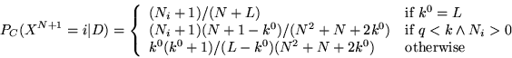
In the case where our knowledge about a domain leads us to specify some
known set of vocabularies
![]() , we can write
, we can write
 |
|||
 |
(3) |
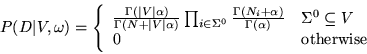
The intuition behind this approach is that it adds to Friedman and Singer's method a second process that attempts to classify the target distribution as one of a number of known distributions, and uses the posterior probability of these distributions for full Bayesian smoothing. However, rather than using the potentially fragile approach of classifying the data based upon the distribution over symbols, the model attempts to classify the data in terms of a set of known vocabularies. Applying standard Bayesian multinomial estimation within each of these vocabularies gives sufficient flexibility for the method to capture a range of distributions, while allowing prior knowledge to play an important role in informing the results.
Text compressiom provides an effective test of methods for multinomial estimation. One approach to adaptive coding involves specifying a method for calculating a distribution over the probability of the next byte in a file based upon the preceding bytes [#!clearywb90!#]. The extent to which the file can be compressed will depend upon the quality of the resulting predictions. This method was explicitly used by Ristad to assess his approach to multinomial estimation, and implicitly used by Friedman and Singer.
To illustrate the utility of including prior knowledge in multinomial
estimation, I will follow Ristad in examining the performance of these
various methods on the Calgary text compression corpus
[#!clearywb90!#]. This corpus consists of 19 files of several different
types, each containing some subset of the 256 possible characters in some
order (
![]() ). The files include BibTeX source (bib), formatted English text
(book1, book2,
paper1, paper2, paper3, paper4, paper5,
paper6), geological data (geo), newsgroup postings ( news), a bit-mapped monochrome picture (pic), programs in three
different languages (progc, progl, progp)
and a terminal transcript (trans). The task was to repeatedly
estimate the multinomial distribution from which characters in the file
were drawn based upon the first
). The files include BibTeX source (bib), formatted English text
(book1, book2,
paper1, paper2, paper3, paper4, paper5,
paper6), geological data (geo), newsgroup postings ( news), a bit-mapped monochrome picture (pic), programs in three
different languages (progc, progl, progp)
and a terminal transcript (trans). The task was to repeatedly
estimate the multinomial distribution from which characters in the file
were drawn based upon the first ![]() characters, and use this
distribution to predict the
characters, and use this
distribution to predict the ![]() st character. Performance was measured
in terms of the length of the resulting file, where the contribution the
st character. Performance was measured
in terms of the length of the resulting file, where the contribution the
![]() st character makes to the length is given by
st character makes to the length is given by
![]() . The
final file length is thus the accumulation of a single term in the cross
entropy of the distribution a method produces for predicting each
successive character, and provides a good measure of the quality of the
estimator for a range of values of
. The
final file length is thus the accumulation of a single term in the cross
entropy of the distribution a method produces for predicting each
successive character, and provides a good measure of the quality of the
estimator for a range of values of ![]() .
.
Text compression is a domain in which files are likely to fall into one
of a small number of categories, so giving extra weight to specific
vocabularies can be of great utility. For the predictions of the
extended Bayesian approach outlined above, the ``known'' vocabularies
corresponded to the characters that occurred in a separate set of files
each containing between 0.5 and 2 megabytes of BibTeX source, English text, C
code, LISP code, and newsgroup postings. The resulting vocabularies
identified 100, 92, 100, 157, and 102 specific characters as belonging
to documents of a particular type. Finally, a vocabulary was added to
cover files that use all 256 characters. Together, these six
vocabularies specified
![]() .
. ![]() was set to
was set to ![]() , as
was done by Friedman and Singer in their experiments with characters. The
text compression results are shown in Table 1.
, as
was done by Friedman and Singer in their experiments with characters. The
text compression results are shown in Table 1.
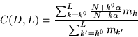
| file | size |
|
|||||||
| bib | 111261 | 81 | 72330 | 79 | 70 | 122 | 92 | 269 | 174 |
| book1 | 768771 | 82 | 435043 | 160 | 151 | 137 | 116 | 352 | 219 |
| book2 | 610856 | 96 | 365952 | 96 | 87 | 167 | 124 | 329 | 212 |
| geo | 102400 | 256 | 72274 | 173 | 172 | 279 | 165 | 165 | 161 |
| news | 377109 | 98 | 244633 | 96 | 86 | 159 | 116 | 304 | 201 |
| obj1 | 21504 | 256 | 15989 | 132 | 136 | 284 | 129 | 129 | 126 |
| obj2 | 246814 | 256 | 193144 | 197 | 190 | 333 | 190 | 189 | 182 |
| paper1 | 53161 | 95 | 33113 | 75 | 66 | 137 | 100 | 236 | 156 |
| paper2 | 82199 | 91 | 47280 | 74 | 65 | 133 | 105 | 259 | 167 |
| paper3 | 46526 | 84 | 27132 | 69 | 61 | 118 | 92 | 238 | 154 |
| paper4 | 13286 | 80 | 7806 | 60 | 51 | 104 | 79 | 190 | 126 |
| paper5 | 11954 | 91 | 7376 | 61 | 53 | 119 | 83 | 181 | 122 |
| paper6 | 38105 | 93 | 23861 | 72 | 63 | 131 | 95 | 223 | 149 |
| pic | 513216 | 159 | 77636 | 138 | 149 | 325 | 216 | 323 | 205 |
| progc | 39611 | 92 | 25743 | 73 | 65 | 131 | 91 | 222 | 150 |
| progl | 71646 | 87 | 42720 | 59 | 65 | 150 | 97 | 253 | 164 |
| progp | 49379 | 89 | 30052 | 72 | 64 | 131 | 94 | 236 | 155 |
| trans | 93695 | 99 | 64800 | 135 | 127 | 145 | 105 | 252 | 169 |
It is instructive to examine the kinds of files on which the Bayesian
method outlined above (![]() ) outperformed the other methods for
multinomial estimation. These files were bib, book1, news, paper1, paper2, paper3, paper4, paper5, paper6, progc, progl, and progp. In these
cases, only
) outperformed the other methods for
multinomial estimation. These files were bib, book1, news, paper1, paper2, paper3, paper4, paper5, paper6, progc, progl, and progp. In these
cases, only ![]() outperformed
outperformed ![]() . These files all use a
restricted vocabulary of characters corresponding to those used in English
text, together with a small number of formatting characters. The high
performance in these cases was a result of the fact that three of the
vocabularies in
. These files all use a
restricted vocabulary of characters corresponding to those used in English
text, together with a small number of formatting characters. The high
performance in these cases was a result of the fact that three of the
vocabularies in
![]() contain such characters - the Bibtex
source, C code, and newsgroup postings. The vocabulary corresponding to
plain English text was too restrictive for most of these files, and was
hardly used, while the vocabulary for Lisp programs was too large to be of
utility. Without this additional structure, Friedman and Singer's method
(
contain such characters - the Bibtex
source, C code, and newsgroup postings. The vocabulary corresponding to
plain English text was too restrictive for most of these files, and was
hardly used, while the vocabulary for Lisp programs was too large to be of
utility. Without this additional structure, Friedman and Singer's method
(
![]() ) tended to perform worse than Ristad's simpler
method (
) tended to perform worse than Ristad's simpler
method (![]() ), although better than the basic Dirichlet smoothing methods
(
), although better than the basic Dirichlet smoothing methods
(![]() and
and ![]() ) when the files used restricted vocabularies.
) when the files used restricted vocabularies.
The results for book1 illustrate an important weakness of the
approach outlined above. Here the file lengths for ![]() and
and
![]() are higher than those for
are higher than those for
![]() and
and ![]() , despite the fact that the file in question features a
restricted English-based vocabulary. The reason for this is that the file
also contains two unusual characters that were not encountered in the data
used to construct any of the specific hypotheses. Upon
encountering these characters
, despite the fact that the file in question features a
restricted English-based vocabulary. The reason for this is that the file
also contains two unusual characters that were not encountered in the data
used to construct any of the specific hypotheses. Upon
encountering these characters ![]() defaulted to the only
defaulted to the only
![]() that contained those characters: the unrestricted vocabulary of
all 256 characters. From that point, the distribution for
that contained those characters: the unrestricted vocabulary of
all 256 characters. From that point, the distribution for ![]() corresponded to Equation
corresponded to Equation ![]() with
with ![]() , and the
resulting smoothing was worse than for
, and the
resulting smoothing was worse than for
![]() and
and ![]() .
.
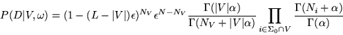
The kind of behaviour that was demonstrated in the compression of book1 is undesirable - we don't want to reject one of our candidate
vocabularies on the basis of one or two symbols that are inconsistent with
that vocabulary. We can improve the robustness of our model by adding in a
noise process such that, regardless of vocabulary, any character in
![]() can occur with some small probability. A direct mixture of
can occur with some small probability. A direct mixture of
![]() with a uniform noise process results in an intractable sum
over all of the
with a uniform noise process results in an intractable sum
over all of the ![]() ways of assigning observations to the smoothed
vocabulary and the noise process, but we can obtain a simple closed form
solution if we assume that the noise process and vocabulary are
mutually exclusive. Assuming that any symbol in
ways of assigning observations to the smoothed
vocabulary and the noise process, but we can obtain a simple closed form
solution if we assume that the noise process and vocabulary are
mutually exclusive. Assuming that any symbol in ![]() occurs with
probability
occurs with
probability ![]() , we have
, we have
The definition of ![]() will determine the upper bound on the
probability mass assigned to the noise distribution. Specifically, this
bound will be given by
will determine the upper bound on the
probability mass assigned to the noise distribution. Specifically, this
bound will be given by ![]() . This gives us a simple heuristic
for setting
. This gives us a simple heuristic
for setting ![]() : if the probability mass that we want to assign to
noise is
: if the probability mass that we want to assign to
noise is ![]() , then we take
, then we take
![]() .
.
While text compression serves as an illustrative domain for the comparison of different parameter estimation techniques, there are a number of other contexts in which we might wish to estimate multinomial distributions about which we have good prior knowledge. One such context is statistical natural language processing, in which accurate multinomial estimation is the topic of much research [#!cheng98!#]. Typically, such multinomial distributions are over large vocabularies of words. Here, the notion of smoothing a multinomial estimate based upon classification of the vocabulary involved has a direct connection to the ideas driving the text classification literature (eg. [#!yang99!#]): in different contexts, words will occur with different probabilities. In particular, different vocabularies will be used, and having a good set of candidate vocabularies may facilitate smoothing. If it is possible to classify a document as using a particular vocabulary, then we can perform smooth the results we obtain appropriately.
A dataset containing a total of approximately 20,000 articles drawn from
20 different Usenet newsgroups was used to examine this idea. This dataset
was first used for text classification in [#!lang95!#], and has since
been a benchmark for text classification algorithms. Ten of these
newsgroups (rec.autos, rec.sport.baseball, sci.crypt,
sci.med, talk.politics.misc, talk.religion.misc, misc.forsale, comp.sys.mac.hardware, comp.os.ms-windows.misc,
comp.graphics) were used to estimate a set of vocabularies
![]() . These vocabularies were then applied in forming multinomial
estimates for further data drawn from these ten newsgroups and ten others
(alt.atheism, sci.space, rec.motorcycles, talk.politics.guns, comp.sys.ibm.pc.hardware, rec.sport.hockey,
. These vocabularies were then applied in forming multinomial
estimates for further data drawn from these ten newsgroups and ten others
(alt.atheism, sci.space, rec.motorcycles, talk.politics.guns, comp.sys.ibm.pc.hardware, rec.sport.hockey,
talk.politics.mideast, sci.electronics,
comp.windows.x).
The actual dataset used was 20news-18827, which consists of the 20
newsgroup data with headers and duplicates removed. The dataset was
preprocessed to remove all punctuation and capitalization, as well as
converting every number to a single symbol. The articles in each of the 20
newsgroups were then divided into three sets. The first set contained the
first 500 articles, and this was used to build the candidate vocabularies
![]() for the ten newsgroups described above. The second set
contained articles 501-700, and was used as training data for multinomial
estimation for all 20 newsgroups. The third set contained articles
701-900, and was used as testing data for all 20 newsgroups. A dictionary
was built up by running over the 13,000 articles resulting from this
division, and all words that occurred only once in this entire reduced
dataset were mapped to an ``unknown'' word. The resulting dictionary
contained
for the ten newsgroups described above. The second set
contained articles 501-700, and was used as training data for multinomial
estimation for all 20 newsgroups. The third set contained articles
701-900, and was used as testing data for all 20 newsgroups. A dictionary
was built up by running over the 13,000 articles resulting from this
division, and all words that occurred only once in this entire reduced
dataset were mapped to an ``unknown'' word. The resulting dictionary
contained ![]() words.
words.
For the generalized Bayesian model discussed above,
![]() featured one vocabulary that contained all words in the dictionary, and 10
vocabularies estimated from each of the 10 newsgroups mentioned
above. These 10 vocabularies were produced by thresholding word frequency
in the 500 articles considered, with the threshold ranging from 1 to 10
instances. Each newsgroup thus provided a hierarchy of vocabularies
representing a range of degrees of specificity.
featured one vocabulary that contained all words in the dictionary, and 10
vocabularies estimated from each of the 10 newsgroups mentioned
above. These 10 vocabularies were produced by thresholding word frequency
in the 500 articles considered, with the threshold ranging from 1 to 10
instances. Each newsgroup thus provided a hierarchy of vocabularies
representing a range of degrees of specificity.
Five methods of multinomial estimation were considered. Since the
candidate vocabularies are simultaneously too general and too specific to
give high probability to any set of observations, ![]() tends to make
no contribution to
tends to make
no contribution to ![]() . For this reason I evaluated
. For this reason I evaluated ![]() and
and
![]() separately. I also considered Ristad's law
(
separately. I also considered Ristad's law
(![]() ), Laplace's law (
), Laplace's law (![]() ) and the Jeffreys-Perks law (
) and the Jeffreys-Perks law (![]() ). For
). For
![]() , the maximum probability mass assigned to noise was
, the maximum probability mass assigned to noise was ![]() ,
while both
,
while both ![]() and
and
![]() used
used ![]() , to
facilitate comparison with the Jeffreys-Perks law.
, to
facilitate comparison with the Jeffreys-Perks law.
Testing for each newsgroup consisted of taking words from the 200 articles
assigned for training purposes, estimating a distribution using each
method, and then computing the cross-entropy between that
distribution and an empirical estimate of the true distribution. The cross
![]() , where
, where ![]() is the true
distribution and
is the true
distribution and ![]() is the distribution produced by the estimation
method. The estimate of
is the distribution produced by the estimation
method. The estimate of ![]() corresponded to the maximum likelihood
estimate formed from the word frequencies in all 200 articles assigned for
testing purposes. The testing procedure was conducted with just 100 words, and
then in increments of 450 words until 10000 words had been seen in
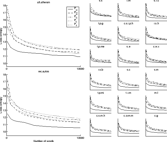
total. The results are shown in Figure 1.
corresponded to the maximum likelihood
estimate formed from the word frequencies in all 200 articles assigned for
testing purposes. The testing procedure was conducted with just 100 words, and
then in increments of 450 words until 10000 words had been seen in
total. The results are shown in Figure 1.
As can be seen in Figure 1, ![]() consistently outperforms the other
methods, even on newsgroups that did not contribute to
consistently outperforms the other
methods, even on newsgroups that did not contribute to
![]() . Performance was worst for sci.space, rec.sport.hockey, and talk.politics.mideast. These newsgroups are
those that showed the least correspondence to those constituting
. Performance was worst for sci.space, rec.sport.hockey, and talk.politics.mideast. These newsgroups are
those that showed the least correspondence to those constituting
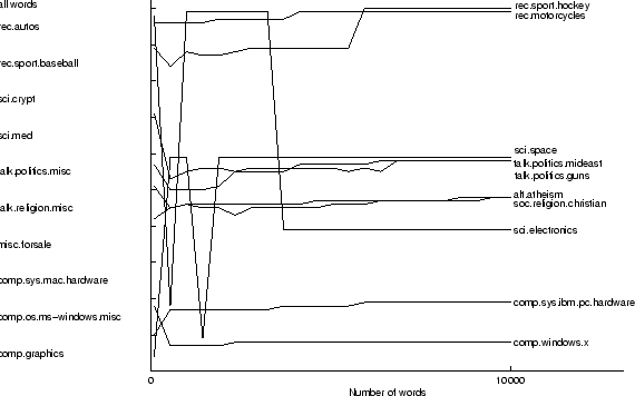
![]() . Figure 2 shows the vocabularies from
. Figure 2 shows the vocabularies from
![]() that
had highest posterior probability at each point in the training
process. sci.space moves between comp.graphics and talk.politics.misc, although neither of these seem to be
appropriate. rec.sport.hockey defaults to the vocabulary containing
all words once the number of unknown words is easier to account for by
this vocabulary than by a noise process combined with the most general
vocabulary in rec.sport.baseball.
that
had highest posterior probability at each point in the training
process. sci.space moves between comp.graphics and talk.politics.misc, although neither of these seem to be
appropriate. rec.sport.hockey defaults to the vocabulary containing
all words once the number of unknown words is easier to account for by
this vocabulary than by a noise process combined with the most general
vocabulary in rec.sport.baseball.
This defaulting behavior is an important aspect of ![]() : at the
point where the data are best accounted for by smoothing on the whole
dictionary, the model will use an unrestricted vocabulary. The resulting
multinomial estimates will be the same as applying Equation
: at the
point where the data are best accounted for by smoothing on the whole
dictionary, the model will use an unrestricted vocabulary. The resulting
multinomial estimates will be the same as applying Equation
![]() with the appropriate setting of
with the appropriate setting of ![]() . In the present
experiment, the
. In the present
experiment, the ![]() parameter was set so that the default estimate
would correspond to
parameter was set so that the default estimate
would correspond to ![]() . This allows a direct evaluation of how much is
being gained by considering restricted vocabularies.
. This allows a direct evaluation of how much is
being gained by considering restricted vocabularies.
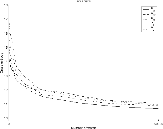
The importance of defaulting is illustrated in Figure 3. After 10,000
words, ![]() is beginning to perform worse than
is beginning to perform worse than ![]() on sci.space. However, if we continue to examine the predictions made by
on sci.space. However, if we continue to examine the predictions made by
![]() as more words are added, we see that the model swiftly defaults
to using
as more words are added, we see that the model swiftly defaults
to using ![]() as soon as the penalty for the unknown words exceeds the
gains of the restricted vocabulary. This is valuable, since at this point
sufficient data have accumulated that
as soon as the penalty for the unknown words exceeds the
gains of the restricted vocabulary. This is valuable, since at this point
sufficient data have accumulated that ![]() gives a good estimate of the
target distribution. The intelligent choice of
gives a good estimate of the
target distribution. The intelligent choice of
![]() is
important to these results. Experiments conducted with 100 vocabularies
generated at random showed very rapid defaulting - the random
vocabularies tended to be strongly inconsistent with the actual data.
is
important to these results. Experiments conducted with 100 vocabularies
generated at random showed very rapid defaulting - the random
vocabularies tended to be strongly inconsistent with the actual data.
The experiment presented above involved estimating only a single
multinomial distribution over words. For tasks like the estimation of
transition probabilities, it becomes necessary to maintain multiple such
estimates. In these cases, the memory demands of an estimation method
become an important concern. Implementing ![]() requires more memory
than doing simple Bayesian smoothing, however the amount of memory
required scales lineary with
requires more memory
than doing simple Bayesian smoothing, however the amount of memory
required scales lineary with
![]() . Since standard Bayesian
smoothing is equivalent to the case where
. Since standard Bayesian
smoothing is equivalent to the case where
![]() , the
resulting cost is not too extreme in most situations.
, the
resulting cost is not too extreme in most situations.
Efficient implementation of ![]() requires storing a list of the
words that belong in each of the
requires storing a list of the
words that belong in each of the
![]() vocabularies, and a
vector of the posterior probabilities of each
vocabularies, and a
vector of the posterior probabilities of each
![]() .
. ![]() can then be evaluated for any given word by taking
a weighted average of the probabilities assigned to that word by applying
standard Bayesian smoothing (Lidstone's law) within that vocabulary. The
time required to compute a probability will thus also increase linearly
with
can then be evaluated for any given word by taking
a weighted average of the probabilities assigned to that word by applying
standard Bayesian smoothing (Lidstone's law) within that vocabulary. The
time required to compute a probability will thus also increase linearly
with
![]() , but when the number of candidate vocabularies
is small the algorithm will remain efficient.
, but when the number of candidate vocabularies
is small the algorithm will remain efficient.
In this paper, I have presented a novel approach to Bayesian smoothing of sparse multinomial distributions. This approach follows the idea of maintaining uncertainty over restricted vocabularies by allowing the vocabularies themselves to be specified on the basis of domain-specific knowledge. I have argued that this approach has its most valuable applications in statistical natural language processing, where data is sparse but domain knowledge is extensive. The main utility of this approach is that if a set of basis vocabularies that span a wide range of contexts can be found, it may be possible to achieve rapid and accurate smoothing of multinomial distributions over words by classifying documents according to their vocabularies.