Finding Syntax with Structural Probes
Human languages, numerical machines
In human languages, the meaning of a sentence is constructed by composing small chunks of words together with each other, obtaining successively larger chunks with more complex meanings until the sentence is formed in its entirety.
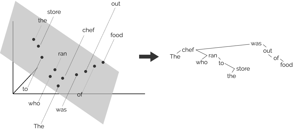
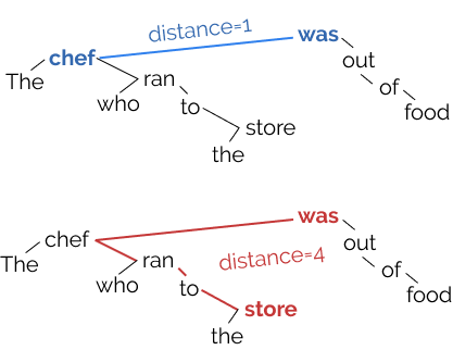
The order in which these chunks are combined creates a tree-structured hierarchy like the one in the picture above (right), which corresponds to the sentence The chef who ran to the store was out of food. Note in this sentence that the store is combined eventually with chef, which then is combined with was, since it is the chef who was out of food, not the store. We refer to each sentence’s tree-sturctured hierarchy as a parse tree, and the phenomenon broadly as syntax.
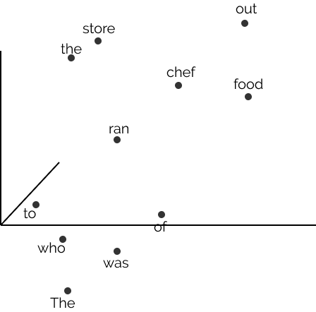
In recent years, however, neural networks used in NLP have represented each word in the sentence as a real-valued vector, with no explicit representation of the parse tree. To these networks, our example sentence looks like the image below (though instead of three-dimensional vectors, they’re more like one thousand dimensions.)

What does the sentence look like in a vector space? Perhaps something like this:
Human languages with tree structures, numerical machines with vector representations. A natural question arises: are these views of language reconcilable?
In this blog post, we’ll explore the vector representations learned by large neural networks like ELMo and BERT, which were simply trained to learn what typical English sentences are like, given a lot of English text. We’ll present a method for finding tree structures in these vector spaces, and show the surprising extent to which ELMo and BERT encode human-like parse trees.
What does this look like? The following image gives an intuition:
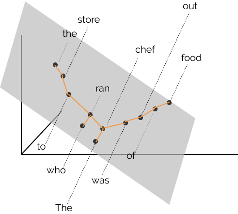
By finding the right linear transformation of the points, we find that the tree constructed by connecting each word to the word closest to it (drawn in yellow) approximates the human parse tree we drew at the top of this article (and the same property holds for many sentences!)
Our method, which we dub a structural probe, is proposed in the forthcoming NAACL 2019 publication, A Structural Probe for Finding Syntax in Word Representations; this post draws from the paper, which is joint work with Chris Manning. The code for the paper, and quick ways of generating graphs like those in this blog post, are found at the structural-probes codebase.
If you want to skip the background and head straight to the discussion of structural probes, go here. Otherwise, let’s jump right into the backstory.
Contextual representations of language
Let’s start by discussing some context about vector representations of language in the last 6 or so years, so we know what we’re analyzing.
The release of pre-trained vector embeddings for word types, as constructed by word2vec or GloVE, led to a wave of research in natural language processing demonstrating their broad utility in various situations. These pre-trained embeddings specify a function which maps elements \(v\) in a (word) vocabulary \(V\) to vectors, \(h\in\mathbb{R}^d\), that is:
\[f_\text{vocab}: v \rightarrow h\]Subword-informed methods like FastText build on the intuition that the literal character sequences of language often are indicative of compositional information about the meaning of the word. These methods map from tuples of vocabulary item \(v\) and character sequence \((c_1,...,c_t)\) to vectors:
\[f_\text{subword}: (v, (c_1,...,c_t)) \rightarrow h\]Contextual representations of language are functions that have yet a more expressive type signature; they leverage the intuition that the meaning of a particular word in a particular text depends not only on the identity of a word, but also on the words that surround it at that moment. Let \((w_1, w_2, .., w_N)\) be a text (say, a sentence) where each \(w_i \in V\) is a word. A contextual representation of language is a function on the whole text, which assigns a vector representation to each word in the sequence:
\[f_\text{contextual}: (w_1,...,w_N) \rightarrow (h_1,...,h_N)\]By a combination of huge datasets, lots of gradient steps, and some smart training strategies, CoVe, ELMo, ULMFiT, GPT, BERT, and GPT2 are considered to build strong contextual representations of language. They differ in many (sometimes meaningful) ways, which we’ll ignore for now.1 These models are trained on objectives that are something along the lines of language modeling, the task of assigning a probability distribution over sequences of words that matches the distribution of a language. (well, except CoVe.)
Beyond “words in context”
Complementary to the “words in context” view of these models’ behavior, it has been suggested that strong contextual models implicitly, softly perform some of the tasks we think are important for true language understanding, e.g., syntax, coreference, question answering. (See Jacob Devlin’s BERT slides, under “Common Questions”; the GPT2 paper).
The suggestion is that in order to perform language modeling well, with enough data, one implicitly has to know seemingly high-level language information. Consider the following first sentence of a story, along with two possible continuations:
The chef who went to the store was out of food.
- Because there was no food to be found, the chef went to the next store.
- After stocking up on ingredients, the chef returned to the restaurant.
The second continuation is much more likely than the first, since it is the chef who is out of food in the premise sentence, not the store. However, the string the store was out of food is a substring of the premise. Thus, knowing that the (chef, was) not the (store, was) may be helpful. More generally, implicitly understanding the syntax of the language may be useful in optimizing the language modeling objective. The dependency parse tree below encodes this intuition.

Next, we’ll go over some thoughts on analysis of neural networks; then we’ll move on to our proposed method for finding syntax in word representations.
What did my neural network learn along the way?
It’s a fun set of hypotheses, “my neural network implicitly learns X phenomenon as it goes about its business optimizing for its objective”, where X is whatever language-related thing you like. Unfortunately, hypotheses like these are hard to formalize and test.
One could evaluate via downstream tasks: We know from various learderboards, among them GLUE, that fine-tuning a big-ole model like BERT on a downstream task tends to improve over training models from scratch on the task itself. However, this does not test a specific hypothesis about what information is encoded in the model, nor is it truly clear what knowledge is necessary for solving any given dataset.
Instead, the analysis-of-NLP-networks literature has sought to test specific hypotheses about what neural networks learn, and how. This work finds itself somewhere in that body of literature; see this foonote \(\rightarrow\)2 for some past work, as well as this one \(\rightarrow\)3 for some work at NAACL this year that will be concurrent with our work.
Observational vs. constructive evidence
Within the analysis literature, we see a rough distinction between observational studies and constructive studies.
Observational evidence
An observational network study evaluates the model at the task it was optimized for, often hand-crafting inputs to determine whether a given desired behavior is observed. A recent example of this is Linzen et al., 2016, which tests (in English) whether language models assign higher probability to the form of a verb that agrees in number with the subject of the sentence than the form that agrees with unrelated words:
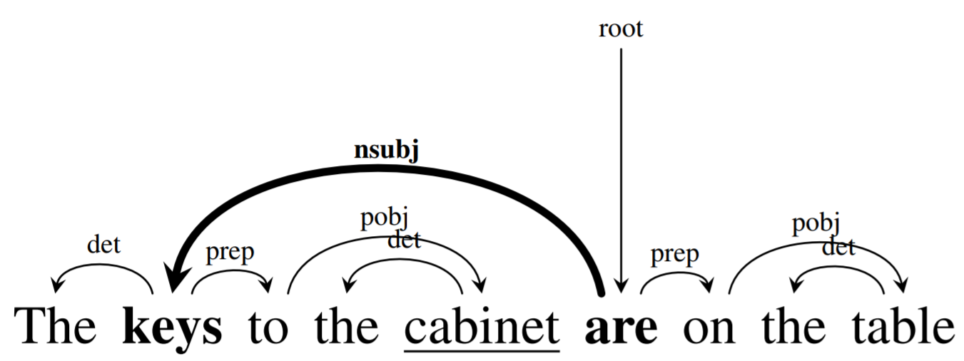
The form of the verb is determined by the head of the subject, which is directly connected to it via an nsubj edge. Other nouns that intervene between the head of the subject and the verb (here cabinet is such a noun) are irrelevant for determining the form of the verb and need to be ignored.
Observational studies are useful because they permit us to ask questions about the model behavior and the data it receives directly, without the confounding factor of a hypothesis about how it achieves its behavior.
Constructive evidence
A constructive study specifies a family of functions, \(\Theta\), by which the model may encode the phenomenon of interest, (syntax, part-of-spech, etc.,) and often then trains on supervised data to choose the member of the family, \(\hat{\theta} \in \Theta\), that best recovers the phenomenon. This is called a probe, or diagnostic classifier.4 A recent example of this is Belinkov et al., 2017, which studies what neural machine translation systems learn about morphology. Their phenomenon of interest was a set of morphological features; their task was cast as a classification task: classify what morphological features hold on each word in each sentence.
They specify 1 hidden-layer feed-forward neural networks as their family of functions by which this information may be encoded in each of the model’s hidden states. That is, they suggest the morphological information \(y_i\) for each word is encoded in the model as:
\[y_i \sim \text{1-layer nn}(h_i)\]for any word \(w_i\), and for some set of parameter values for 1-layer neural networks.
Constructive studies are useful because they permit us constructive evidence for a phenomenon – that is, if our hypothesis is correct, then \(\hat{\theta}\) both provides evidence for the hypothesis and is a way to extract the phenomenon of interest from the underlying model. However, they do not answer the initial question, “does my model learn X phenomenon”; they only answer the proxy question, “does my model encode X phenomenon in a manner extractable by my probe?” Also see a good set of tweets + corresponding NAACL paper preprint by Naomi Saphra which discuss related considerations.
With this, we’re ready to discuss our structural probe work!
The structural probe
Our structural probe tests a simple hypothesis for how parse trees may be embedded in the hidden states of a neural network.
We think of there existing a latent parse tree on every sentence, which the neural network does not have access to.
For the dependency parsing formalisms, each word in the sentence has a corresponding node in the parse tree:
Going back to our earlier example, dependency parse trees look like this:
Trees as distances and norms
The key difficulty is in determining whether the parse tree, a discrete structure, is encoded in the sequence of continuous vectors. Our first intuition is that vector spaces and graphs both have natural distance metrics. For a parse tree, we have the path metric, \(d(w_i,w_j)\), which is the number of edges in the path between the two words in the tree.
With all \(N^2\) distances for a sentence, one can reconstruct the (undirected) parse tree simply by recognizing that all words with distance 1 are neighbors in the tree. Thus, embedding the tree reduces to embedding the distance metric defined by the tree. (We’ll discuss the directions to the edges later.)
So, as a thought experiment, what if it happened to be the case that distance between word vectors constructed by a neural network for a sentence happened to equal the path distance between the words in the latent parse tree? This would be rather convincing evidence that the network had implictly learned to embed the tree. Our structural probe relaxes this requirement somewhat; of course, neural networks have to encode a lot of information in the hidden states, not just syntax, so distance on the whole vector may not make sense. From this, we get the syntax distance hypothesis:
The syntax distance hypothesis: There exists a linear transformation \(B\) of the word representation space under which vector distance encodes parse trees.
Equivalently, there exists an inner product on the word representation space such that distance under the inner product encodes parse trees. This (indefinite) inner product is specified by \(B^TB\) .
We’ll take a particular instance of this hypothesis for our probes; we’ll use the L2 distance, and let the squared vector distances equal the tree distances, but more on this later.
The distances we pointed out earlier between chef, store and was, can be visualized in a vector space as follows, where \(B \in \mathbb{R}^{2\times 3}\), mapping 3-dimensional word representations to a 2-dimensional space encoding syntax:
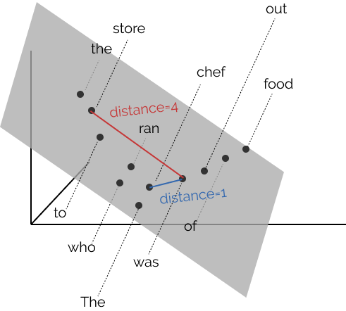
Note in the image above that the distances between words before transformation by \(B\) aren’t indicative of the tree. After the linear transformation, however, taking a minimum spanning tree on the distances recovers the tree, as shown in the following image:
Finding a parse tree-encoding distance metric
Our potentially tree-encoding distances are parametrized by the linear transformation \(B \in \mathbb{R}^{k \times n}\),
\[\|h_i - h_j\|_{B}^2 = (B(h_i - h_j))^T (B(h_i-h_j))\]where \(Bh\) is the linear transformation of the word representation; equivalently, it is the parse tree node representation. This is equivalent to finding an L2 distance on the original vector space, parametrized by the positive semi-definite matrix \(A=B^TB\):
\[\|h_i - h_j\|_{A}^2 = (h_i - h_j)^T A (h_i-h_j)\]The set of linear transformations, \(\mathbb{R}^{k \times n}\) for a given \(k\) is the hypothesis class for our probing family. We choose \(B\) to minimize the difference between true parse tree distances from a human-parsed corpus and the predicted distances from the fixed word representations transformed by \(B\):
\[\min_B \sum_{\ell} \frac{1}{|s_\ell|^2}\sum_{i,j} \big(d(w_i,w_j) - \|B(h_i - h_j)\|^2\big)\]where \(\ell\) indexes the sentences \(s_\ell\) in the corpus, and \(\frac{1}{|s_\ell|^2}\) normalizes for the number of pairs of words in each sentence. Note that we do actually attempt to minimize the difference between the squared distance \(\|h_i-h_j\|_B^2\) and the tree distance. This means that the actual vector distance \(\|h_i-h_j\|_B\) will always be off from the true parse tree distances, but the tree information encoded is identical, and we found that optimizing with the squared distance performs considerably better in practice.5
Finding a parse depth-encoding norm
As a second application of our method, we note that the directions of the edges in a parse tree is determined by the depth of words in the parse tree; the deeper node in the governance relationship is the governed word. The depth in the parse tree is like a norm, or length, defining a total order on the nodes in the tree. We denote this tree depth norm \(\|w_i\|\).
Likewise, vector spaces have natural norms; our hypothesis for norms is that there exists a linear transformation under which tree depth norm is encoded by the squared L2 vector norm \(\|Bh_i\|_2^2\). Just like for the distance hypothesis, we can find the linear transformation under which the depth norm hypothesis is best-approximated:
\[\min_B \sum_{\ell} \frac{1}{|s_\ell|}\sum_{i} \big(\|w_i\| - \|Bh_i\|^2\big)\]Evaluation and Visualization
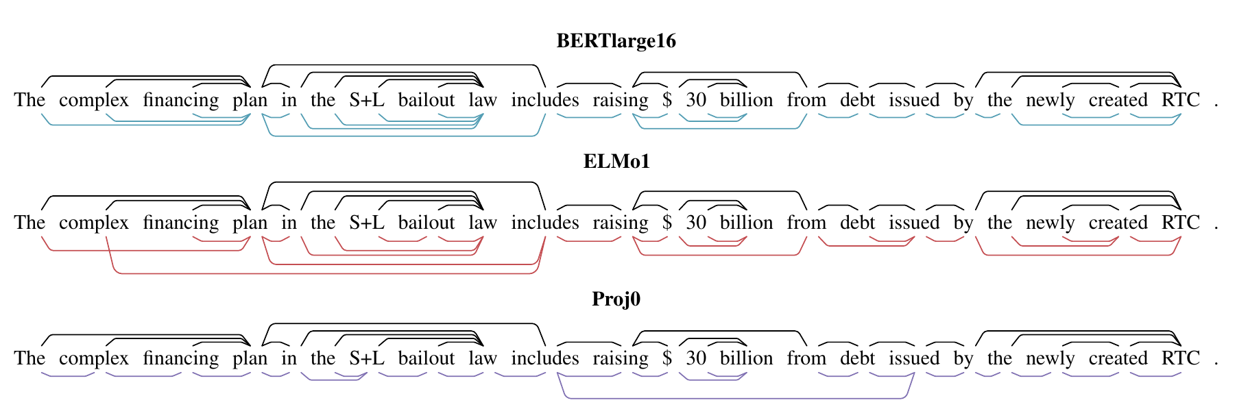
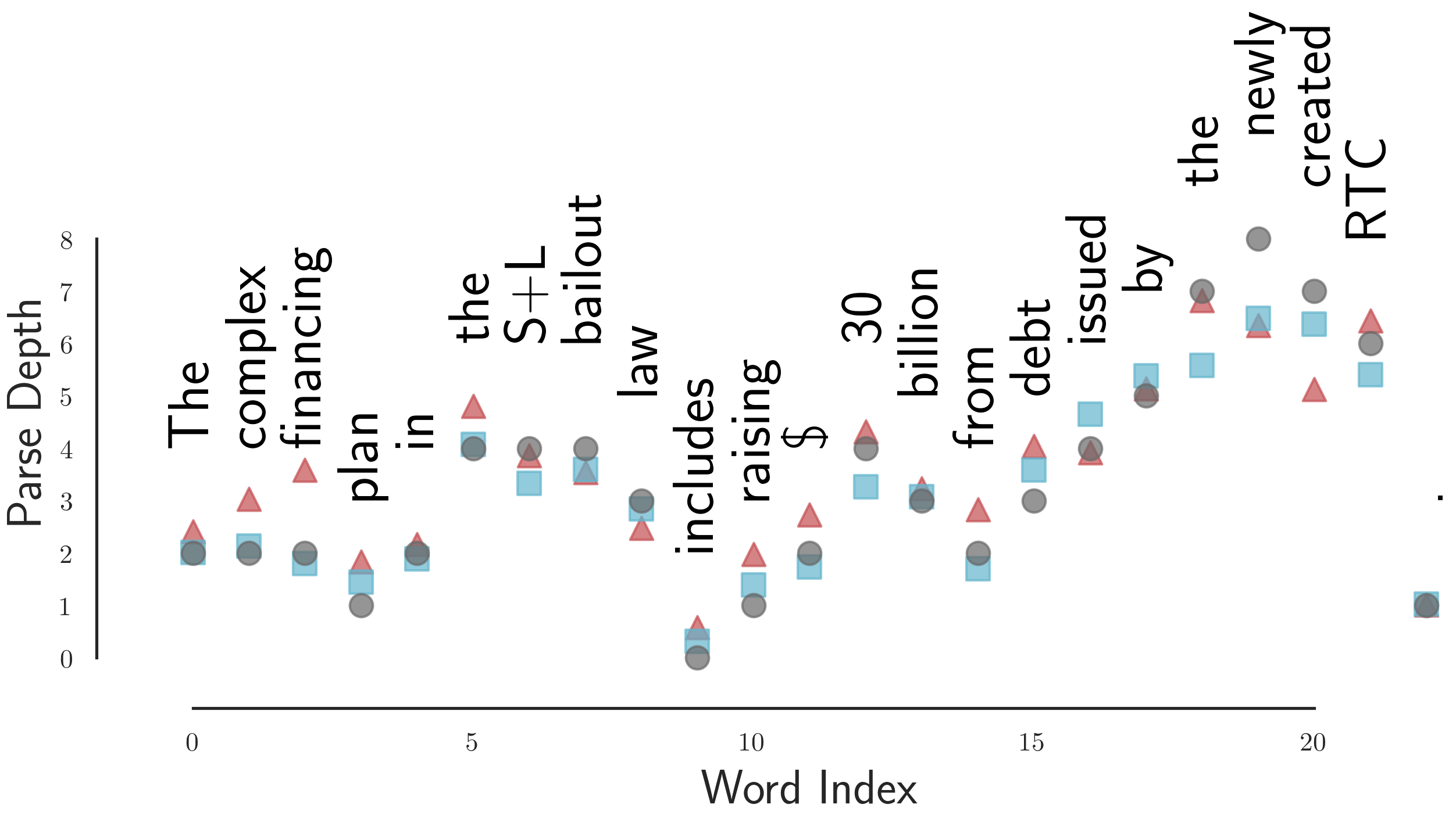
In our paper, we evaluate ELMo and BERT embeddings, as well as a number of baseline methods, on their ability to reconstruct parse trees from the Penn Treebank according to our hypotheses. We evaluate each of the hidden layers of the models separately, denoted for example ELMo0, ELMo1, ELMo2.
ELMo0 is the simplest baseline: each word receives an uncontextualized character-level word embedding. We also evaluate Decay0 and Proj0, two simple ways of contextualizing the word embeddings which cannot be said to “learn to parse”; more details are discussed in the paper.
In this blog post, we’ll focus on giving a qualitative idea of the results; see the paper for quantitative details. The short story is that we were surprised by the quality of syntax-encoding distances and norms we were able to find for both ELMo and BERT!
Reconstructed trees and depths
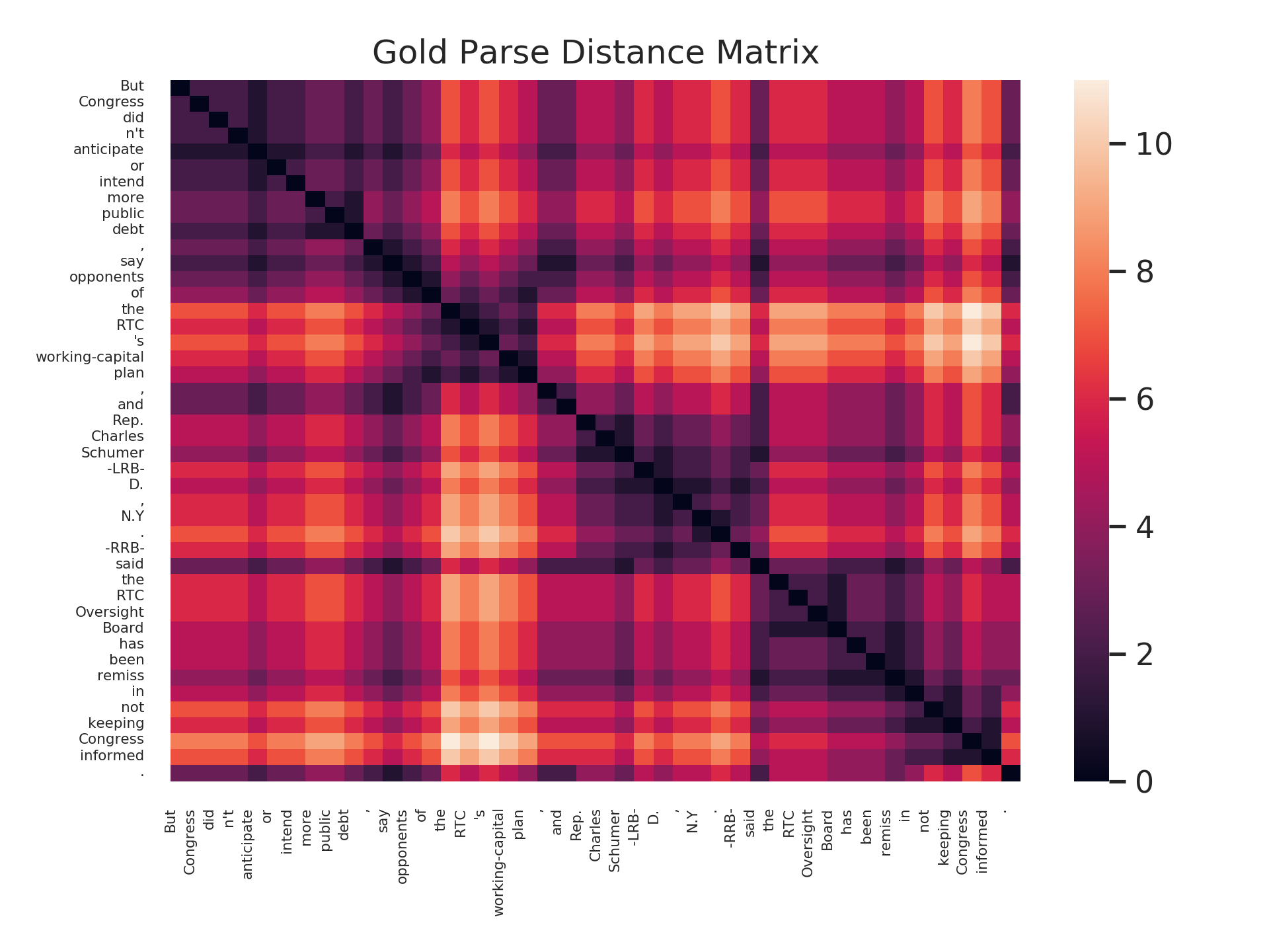
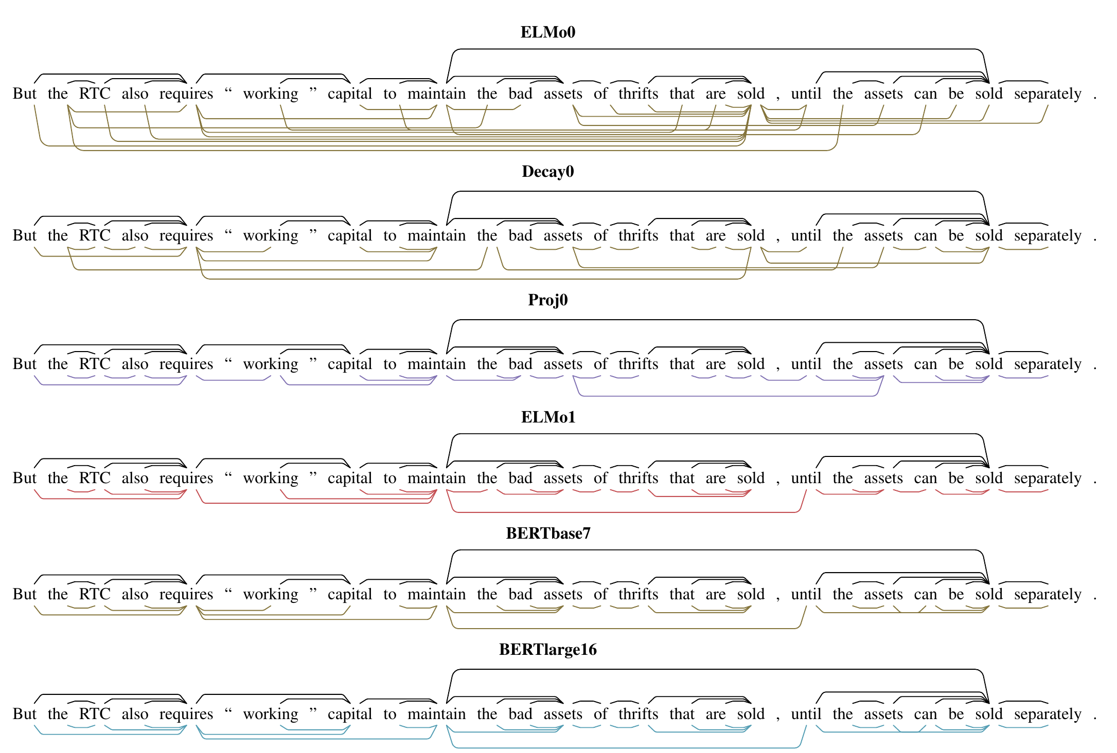
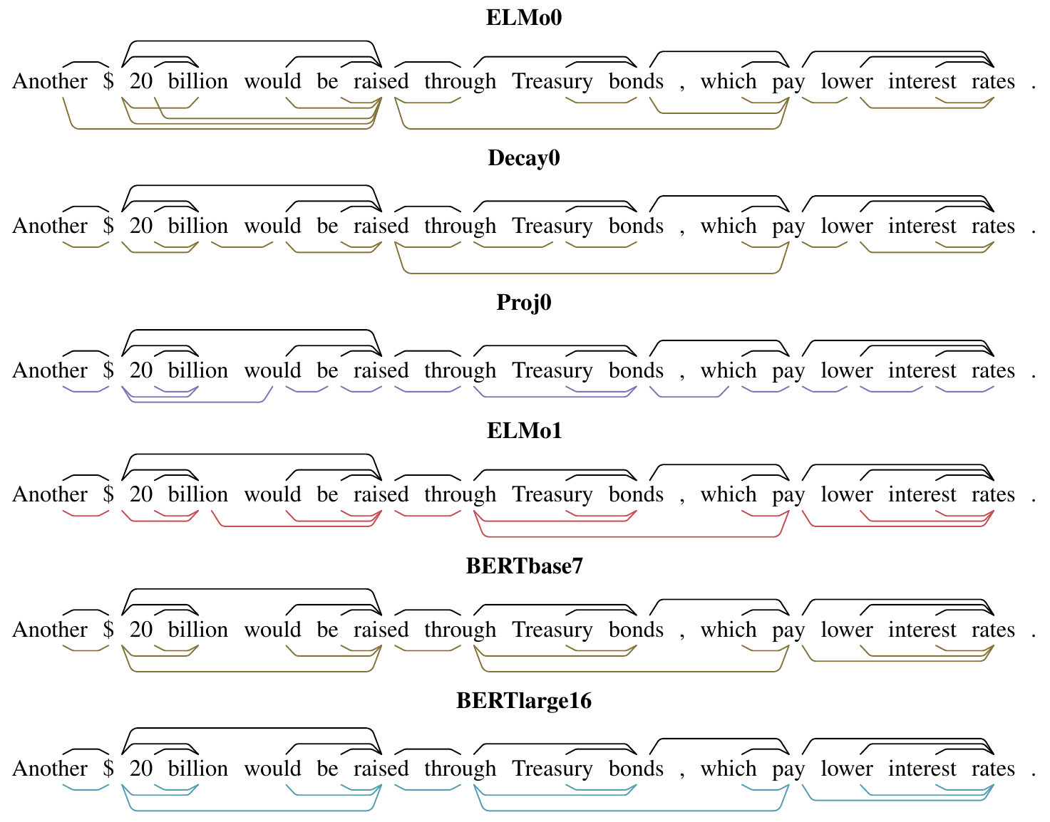
Here, we present a taste of the results through reconstructed trees and tree depths for a number of sentences; these figures are direct from the paper.
First, we see gold parse trees (black, above the sentences) along with the minimum spanning trees of predicted distance metrics for a sentence (blue, red, purple, below the sentence):
Next, we see depths in the gold parse tree (grey, circle) as well as predicted (squared) parse depths according to ELMo1 (red, triangle) and BERT-large, layer 16 (blue, square).
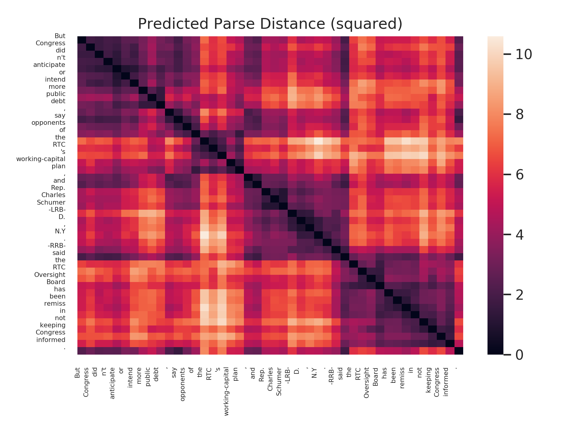
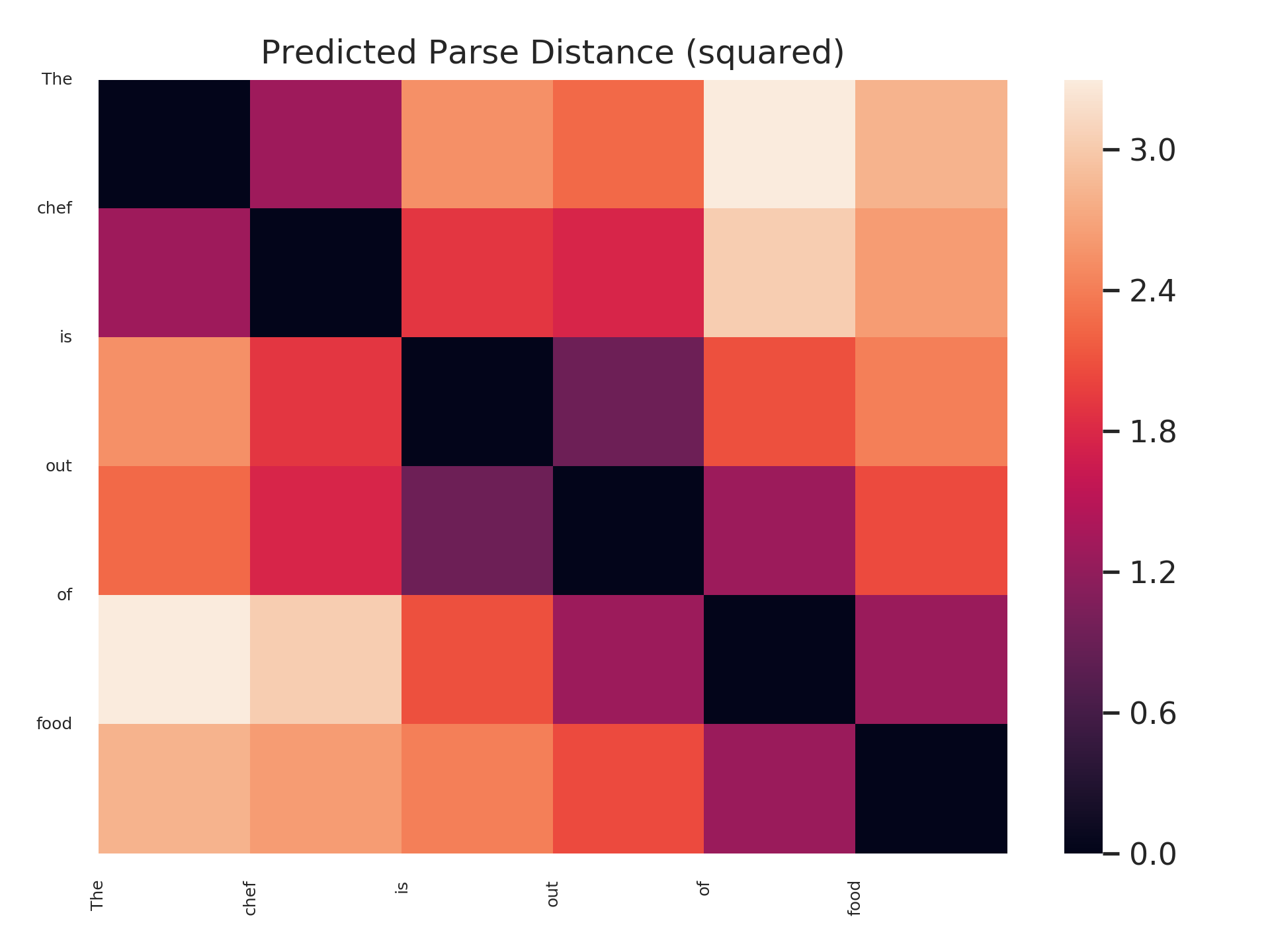
Finally, let’s see the rich structure in a parse distance matrix, which visualizes all pairs of distances between words in a sentence.
Below are both the distance defined by the actual tree, as well as the squared distance according to our probe on BERT-large, layer 16.
Long distances are ligher colors; short distances are darker colors.
A brief example on subject-verb number agreement
For our last inquiry, let’s return to the concept of subject-verb number agreement. This classic test for hierarchy reasons that even as increasing numbers of nouns intervene between a verb and its subject, the verb should still agree in number with its subject, not with the intervening nouns.
In observational studies, one can test this by presenting a language model with a sentence with a (singular) subject and intervening (plural) nouns, and then ask the language model whether the singular or plural form of the verb is higher likelihood given the prefix of the sentence. Language models demonstrate the ability to assign higher conditional probability to the correct form of the verb (Kunkoro et al., 2018;Gulordova et al., 2018).
By the parse tree distance formulation, this subject-verb agreement behavior can be explained by noting that the subject and the verb are at distance 1, whereas the verb and every intervening noun are at greater distances.
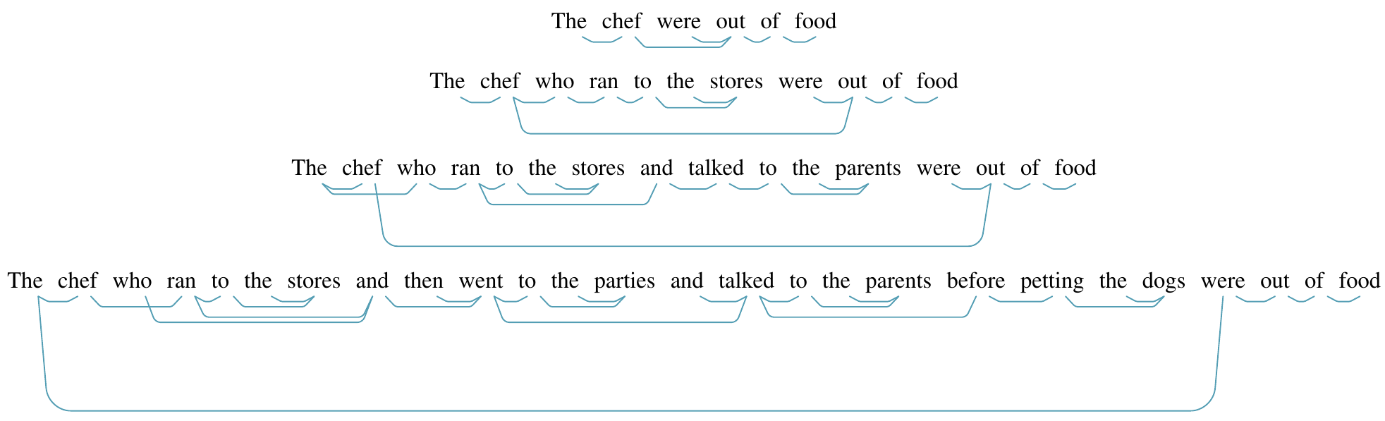
Does this bear out in our trained probes? We leave a comprehensive study of this question for future work, but offer here a visualization suggesting that it is possible! (To be clear, we don’t claim that this question is the same as the original subject-verb number agreement question; the model has access to the correct form of the verb, for example.) Below are distance matrices and minimum spanning trees predicted by a structural probe on BERT-large, layer 16, for 4 sentences. Each sentence adds new “attractor” intervening plural nouns between the subject and the verb.
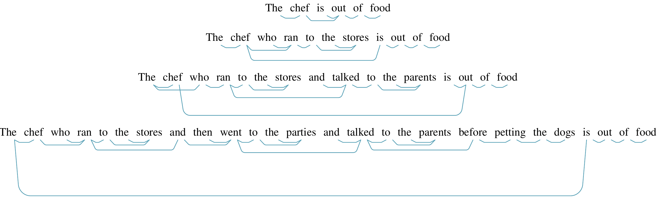
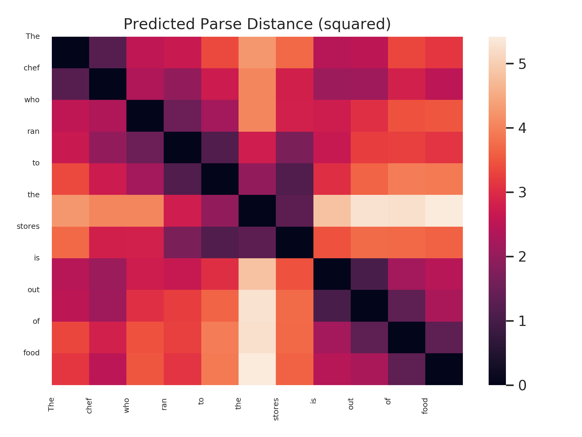
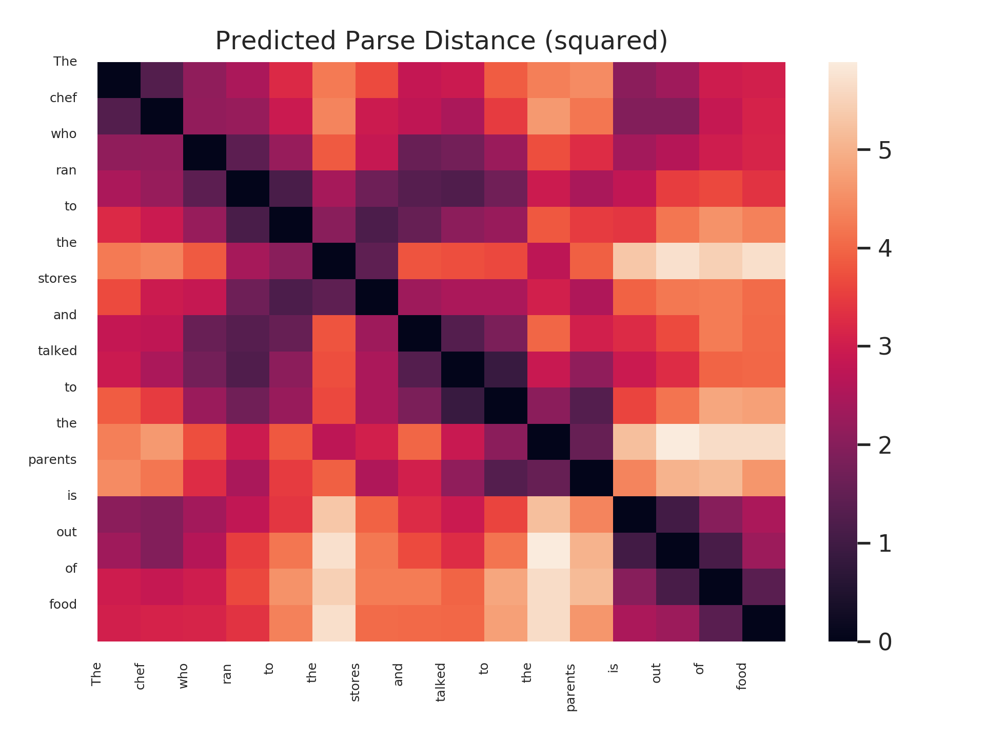
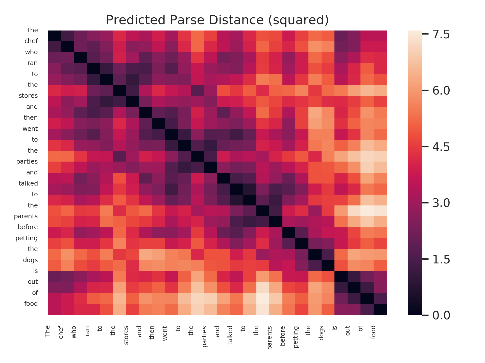
As can be seen, the parse trees are not correct in an absolute sense – a parser, for example, would never attach the word “the” to a verb. However, the desired behavior – subjects and verbs close, even with many intervening nouns – bears out!
As a quick curiosity: what happens when we give BERT and the structural probe an ungrammatical sentence, where the form of the verb given is plural, but still must refer back to a singular subject? We still see largely the same behavior, meaning the model may not just be matching the verb with the noun in the sentence of the same number:
Conclusion
I think it’s pretty exciting that the geometry of English parse trees is approximately discoverable in the geometry of deep models of language. We hope that the targeted case studies we’ve run on BERT and ELMo will be just the start of a wide range of inquiry into the syntactic properties of the geometry of contextualized word representations. Beyond this, dependency syntax is not the only graph structure one might try to find in a linear transformation of a hidden state space; we look forward to work finding other graph structures as well.
If you’d like to run some tests of your own, we have pre-trained probes and bindings for BERT-large which will auto-generate plots like the ones you’ve seen in this blog post in the structural probes codebase.
Many thanks go out to the Stanford NLP group and others for an amazing amount of help received on this work; of course Chris Manning, but also Percy Liang, Urvashi Khandelwal, Tatsunori Hashimoto, Abigail See, Kevin Clark, Siva Reddy, Drew A. Hudson, and Roma Patel.
Extra visualizations
In this next sentence, we see a broader range of models, and see clearly that our probe can’t learn to parse on top of an uncontextualized representation like ELMo0:
 This next sentence is relatively simple, so the differences between the models are subtler.
Footnotes
-
The most salient destinction between these models may be that some are true language models, assigning probability distributions to sequences and thus requiring some chain-rule decomposition that restricts the context available to, say, sentencep refixes. Thus, their type signature is more like \(f_\text{LM}(w_1,...,w_n) \rightarrow h_n\). ↩
-
(Linzen et al, 2016), (Gulordova et al., 2018), (Kuncoro et al., 2018), (Peters et al., 2019b) ↩
-
(Saphra and Lopez, 2019) (Liu et al., 2019) There are definitely more… let me know if you have a recent analysis paper that you think I should add! ↩
-
See Tenney et al., 2019 for example usage of the term “Probing”, and Hupkes et al., 2018 for example usage of “diagnostic classifiers”. ↩
-
See the NAACL paper for more details! ↩