Perhaps the
best-known way of computing good class boundaries is Rocchio
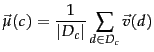
classification , which uses centroids to
define the boundaries. The centroid of
a class ![]() is computed as the vector average or center of
mass of its members:
is computed as the vector average or center of
mass of its members:
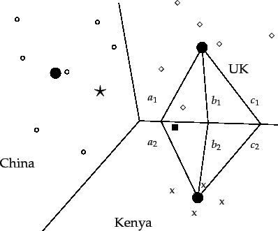
The boundary between two classes in Rocchio
classification is the set of points with equal distance
from the two centroids. For example, ![]() ,
,
![]() , and
, and ![]() in the figure. This set
of points is always a line.
The generalization of a line in
in the figure. This set
of points is always a line.
The generalization of a line in
![]() -dimensional space is
a hyperplane, which we define as the set of points
-dimensional space is
a hyperplane, which we define as the set of points ![]() that satisfy:
that satisfy:
Thus, the boundaries of class regions in Rocchio
classification are hyperplanes. The classification rule in
Rocchio is to
classify a point in accordance with the
region it falls into. Equivalently, we determine the
centroid
![]() that the point is closest to and then assign it to
that the point is closest to and then assign it to ![]() .
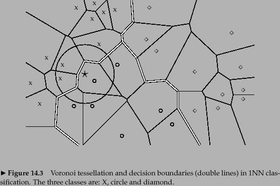
As an example, consider the star
in Figure 14.3 . It is located in the
China region of the space and Rocchio therefore assigns it to China.
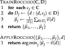
We show the Rocchio algorithm
in pseudocode in
Figure 14.4 .
.
As an example, consider the star
in Figure 14.3 . It is located in the
China region of the space and Rocchio therefore assigns it to China.
We show the Rocchio algorithm
in pseudocode in
Figure 14.4 .
| |||||||||||||||||||||||||||||||||||||||||||||||||||||||||||||||
Worked example.
Table 14.1 shows the tf-idf vector representations of the
five documents in
Table 13.1
(page 13.1 ), using the formula
![]() if
if
![]() (Equation 29, page 6.4.1 ).
The two class centroids are
(Equation 29, page 6.4.1 ).
The two class centroids are
![]() and
and
![]() .
The distances of the test document from the centroids are
.
The distances of the test document from the centroids are
![]() and
and
![]() . Thus, Rocchio
assigns
. Thus, Rocchio
assigns ![]() to
to ![]() .
.
The separating hyperplane in this case has the following parameters:
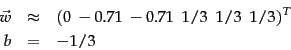
End worked example.
The assignment criterion in
Figure 14.4 is Euclidean distance (APPLYROCCHIO, line 1). An
alternative is cosine similarity:
| (141) |
Rocchio classification is a form of Rocchio relevance
feedback (Section 9.1.1 , page 9.1.1 ). The
average of the relevant documents, corresponding to the most
important component of the Rocchio vector in relevance
feedback (Equation 49, page 49 ), is
the centroid of the ``class'' of relevant documents. We omit
the query component of the Rocchio formula in Rocchio
classification since there is no query in text
classification. Rocchio classification can be applied to
![]() classes whereas Rocchio relevance feedback is designed
to distinguish only two classes, relevant and nonrelevant.
classes whereas Rocchio relevance feedback is designed
to distinguish only two classes, relevant and nonrelevant.
In addition to respecting contiguity, the classes in Rocchio classification must be approximate spheres with similar radii. In Figure 14.3 , the solid square just below the boundary between UK and Kenya is a better fit for the class UK since UK is more scattered than Kenya. But Rocchio assigns it to Kenya because it ignores details of the distribution of points in a class and only uses distance from the centroid for classification.
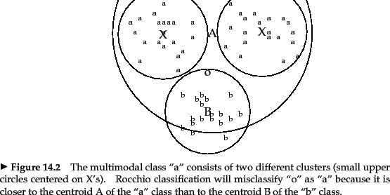
The assumption of sphericity also does not hold in Figure 14.5 . We cannot represent the ``a'' class well with a single prototype because it has two clusters. Rocchio often misclassifies this type of multimodal class . A text classification example for multimodality is a country like Burma, which changed its name to Myanmar in 1989. The two clusters before and after the name change need not be close to each other in space. We also encountered the problem of multimodality in relevance feedback (Section 9.1.2 , page 9.1.3 ).
Two-class classification is another case where
classes are rarely distributed like
spheres with similar radii. Most two-class classifiers
distinguish between a class like China that occupies
a small region of the space and its
widely scattered complement. Assuming equal radii will
result in a large number of false positives. Most
two-class classification problems therefore require a modified
decision rule of the form:
| (142) |
| mode | time complexity |
| training |
|
| testing |
|
Table 14.2 gives the time complexity of Rocchio
classification.![]() Adding all documents to their respective (unnormalized) centroid is
Adding all documents to their respective (unnormalized) centroid is
![]() (as opposed to
(as opposed to
![]() ) since we need
only consider non-zero entries.
Dividing each vector sum by the size of its class to compute
the centroid is
) since we need
only consider non-zero entries.
Dividing each vector sum by the size of its class to compute
the centroid is ![]() .
Overall, training time is
linear in the size of the collection
(cf. Exercise 13.2.1 ). Thus, Rocchio
classification and Naive Bayes have the same linear training
time complexity.
.
Overall, training time is
linear in the size of the collection
(cf. Exercise 13.2.1 ). Thus, Rocchio
classification and Naive Bayes have the same linear training
time complexity.
In the next section, we will introduce another vector space classification method, kNN, that deals better with classes that have non-spherical, disconnected or other irregular shapes.
Exercises.