Centroid clustering

In centroid clustering, the similarity of two clusters is defined as the similarity of their centroids:

$$\mbox{{\sc sim-cent}}(\omega_i,\omega_j) = \vec{\mu}( \omega_i ) \cdot \vec{\mu}( \omega_j )$$ (207)

$$= (\frac{1}{N_i}\sum_{d_\mthatwask \in \omega_i} \vec{d}_\mthatwask) \cdot (\frac{1}{N_j}\sum_{d_\nthatwasell \in \omega_j} \vec{d}_\nthatwasell)$$ (208)

$$= \frac{1}{N_iN_j} \sum_{d_\mthatwask \in \omega_i} \sum_{d_\nthatwasell \in \omega_j} \vec{d}_\mthatwask \cdot \vec{d}_\nthatwasell$$ (209)

Equation 207 is centroid similarity. Equation 209 shows that centroid similarity is equivalent to average similarity of all pairs of documents from different clusters. Thus, the difference between GAAC and centroid clustering is that GAAC considers all pairs of documents in computing average pairwise similarity (Figure 17.3 , (d)) whereas centroid clustering excludes pairs from the same cluster (Figure 17.3 , (c)).

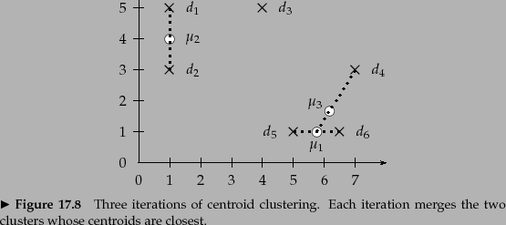
Figure 17.11 shows the first three steps of a centroid clustering. The first two iterations form the clusters $\{d_5,d_6\}$ with centroid $\mu_1$ and $\{d_1,d_2\}$ with centroid $\mu_2$ because the pairs $\langle d_5,d_6 \rangle$ and $\langle d_1,d_2 \rangle$ have the highest centroid similarities. In the third iteration, the highest centroid similarity is between $\mu_1$ and $d_4$ producing the cluster $\{d_4,d_5,d_6\}$ with centroid $\mu_3$.

Like GAAC, centroid clustering is not best-merge persistent and therefore $\Theta(N^2 \log N)$ (Exercise 17.10 ).

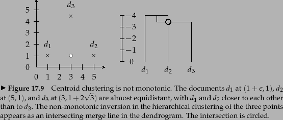
In contrast to the other three HAC algorithms, centroid clustering is not monotonic. So-called inversions can occur: Similarity can increase during clustering as in the example in Figure 17.12 , where we define similarity as negative distance. In the first merge, the similarity of $d_1$ and $d_2$ is $-(4-\epsilon)$. In the second merge, the similarity of the centroid of $d_1$ and $d_2$ (the circle) and $d_3$ is $\approx -\cos(\pi/6)\times 4=-\sqrt{3}/2 \times 4 \approx -3.46>-(4-\epsilon)$. This is an example of an inversion: similarity increases in this sequence of two clustering steps. In a monotonic HAC algorithm, similarity is monotonically decreasing from iteration to iteration.

Increasing similarity in a series of HAC clustering steps contradicts the fundamental assumption that small clusters are more coherent than large clusters. An inversion in a dendrogram shows up as a horizontal merge line that is lower than the previous merge line. All merge lines in and 17.5 are higher than their predecessors because single-link and complete-link clustering are monotonic clustering algorithms.

Despite its non-monotonicity, centroid clustering is often used because its similarity measure - the similarity of two centroids - is conceptually simpler than the average of all pairwise similarities in GAAC. Figure 17.11 is all one needs to understand centroid clustering. There is no equally simple graph that would explain how GAAC works.

Exercises.

• For a fixed set of $N$ documents there are up to $N^2$ distinct similarities between clusters in single-link and complete-link clustering. How many distinct cluster similarities are there in GAAC and centroid clustering?