Queries as vectors

There is a far more compelling reason to represent documents as vectors: we can also view a query as a vector. Consider the query $q=$ jealous gossip. This query turns into the unit vector $\vec{v}(q)=(0,0.707,0.707)$ on the three coordinates of Figures 6.12 and 6.13. The key idea now: to assign to each document $d$ a score equal to the dot product

$$\vec{v}(q)\cdot\vec{v}(d).$$ (26)

In the example of Figure 6.13, Wuthering Heights is the top-scoring document for this query with a score of 0.509, with Pride and Prejudice a distant second with a score of 0.085, and Sense and Sensibility last with a score of 0.074. This simple example is somewhat misleading: the number of dimensions in practice will be far larger than three: it will equal the vocabulary size $M$.

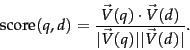
To summarize, by viewing a query as a ``bag of words'', we are able to treat it as a very short document. As a consequence, we can use the cosine similarity between the query vector and a document vector as a measure of the score of the document for that query. The resulting scores can then be used to select the top-scoring documents for a query. Thus we have

$$\mbox{score}(q,d)= \frac{\vec{V}(q)\cdot \vec{V}(d)}{\vert\vec{V}(q)\vert \vert\vec{V}(d)\vert}.$$ (27)

A document may have a high cosine score for a query even if it does not contain all query terms. Note that the preceding discussion does not hinge on any specific weighting of terms in the document vector, although for the present we may think of them as either tf or tf-idf weights. In fact, a number of weighting schemes are possible for query as well as document vectors, as illustrated in Example 6.3.2 and developed further in Section 6.4 .

Computing the cosine similarities between the query vector and each document vector in the collection, sorting the resulting scores and selecting the top $K$ documents can be expensive -- a single similarity computation can entail a dot product in tens of thousands of dimensions, demanding tens of thousands of arithmetic operations. In Section 7.1 we study how to use an inverted index for this purpose, followed by a series of heuristics for improving on this.

Worked example. We now consider the query best car insurance on a fictitious collection with $N=1{,}000{,}000$ documents where the document frequencies of auto, best, car and insurance are respectively 5000, 50000, 10000 and 1000.

term	query				document			product
	tf	df	idf	$\mbox{w}_{t,q}$	tf	wf	$\mbox{w}_{t,d}$
auto	0	5000	2.3	0	1	1	0.41	0
best	1	50000	1.3	1.3	0	0	0	0
car	1	10000	2.0	2.0	1	1	0.41	0.82
insurance	1	1000	3.0	3.0	2	2	0.82	2.46

In this example the weight of a term in the query is simply the idf (and zero for a term not in the query, such as auto); this is reflected in the column header $\mbox{w}_{t,q}$ (the entry for auto is zero because the query does not contain the termauto). For documents, we use tf weighting with no use of idf but with Euclidean normalization. The former is shown under the column headed wf, while the latter is shown under the column headed $\mbox{w}_{t,d}$. Invoking (23) now gives a net score of $0+0+0.82+2.46 = 3.28$. End worked example.