Typical objective functions in clustering formalize the goal of attaining high intra-cluster similarity (documents within a cluster are similar) and low inter-cluster similarity (documents from different clusters are dissimilar). This is an internal criterion for the quality of a clustering. But good scores on an internal criterion do not necessarily translate into good effectiveness in an application. An alternative to internal criteria is direct evaluation in the application of interest. For search result clustering, we may want to measure the time it takes users to find an answer with different clustering algorithms. This is the most direct evaluation, but it is expensive, especially if large user studies are necessary.
As a surrogate for user judgments, we can use a set of classes in an evaluation benchmark or gold standard (see Section 8.5 , page 8.5 , and Section 13.6 , page 13.6 ). The gold standard is ideally produced by human judges with a good level of inter-judge agreement (see Chapter 8 , page 8.1 ). We can then compute an external criterion that evaluates how well the clustering matches the gold standard classes. For example, we may want to say that the optimal clustering of the search results for jaguar in Figure 16.2 consists of three classes corresponding to the three senses car, animal, and operating system. In this type of evaluation, we only use the partition provided by the gold standard, not the class labels.
This section introduces four external criteria of clustering quality. Purity is a simple and transparent evaluation measure. Normalized mutual information can be information-theoretically interpreted. The Rand index penalizes both false positive and false negative decisions during clustering. The F measure in addition supports differential weighting of these two types of errors.
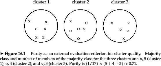
To compute purity ,
each cluster is assigned to the class which is most
frequent in the cluster, and then the accuracy of this
assignment is measured by counting the number of correctly
assigned documents and dividing by ![]() . Formally:
. Formally:
We present an example of how to compute purity in
Figure 16.4 .![]() Bad
clusterings have purity values close to 0, a perfect
clustering has a purity of 1 . Purity is compared with the other three
measures discussed in this chapter in Table 16.2 .
Bad
clusterings have purity values close to 0, a perfect
clustering has a purity of 1 . Purity is compared with the other three
measures discussed in this chapter in Table 16.2 .
|
High purity is easy to achieve when the number of clusters is large - in particular, purity is 1 if each document gets its own cluster. Thus, we cannot use purity to trade off the quality of the clustering against the number of clusters.
A measure that allows us to make this tradeoff is
normalized mutual
information or NMI :
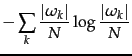
![]() is entropy as defined in Chapter 5
(page 5.3.2 ):
is entropy as defined in Chapter 5
(page 5.3.2 ):
| (186) | |||
 |
(187) |
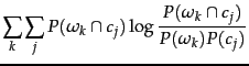
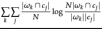
![]() in Equation 184 measures the
amount of information by which our knowledge about the
classes increases when we are told what the clusters are.
The minimum of
in Equation 184 measures the
amount of information by which our knowledge about the
classes increases when we are told what the clusters are.
The minimum of
![]() is 0 if the
clustering is random with respect to class membership. In that
case, knowing that a document is in a particular cluster
does not give us any new information about what its class
might be. Maximum mutual information is reached for a
clustering
is 0 if the
clustering is random with respect to class membership. In that
case, knowing that a document is in a particular cluster
does not give us any new information about what its class
might be. Maximum mutual information is reached for a
clustering
![]() that perfectly recreates the
classes - but also if clusters in
that perfectly recreates the
classes - but also if clusters in
![]() are
further subdivided into smaller clusters
(Exercise 16.7 ). In particular, a clustering
with
are
further subdivided into smaller clusters
(Exercise 16.7 ). In particular, a clustering
with ![]() one-document clusters has maximum MI. So MI has
the same problem as purity: it does not penalize large
cardinalities and thus does not formalize our bias that,
other things being equal, fewer clusters are better.
one-document clusters has maximum MI. So MI has
the same problem as purity: it does not penalize large
cardinalities and thus does not formalize our bias that,
other things being equal, fewer clusters are better.
The normalization by the denominator
![]() in Equation 183 fixes this problem since entropy
tends to increase with the number of clusters. For example,
in Equation 183 fixes this problem since entropy
tends to increase with the number of clusters. For example,
![]() reaches its maximum
reaches its maximum ![]() for
for ![]() , which
, which
ensures that NMI is low for ![]() . Because NMI is
normalized, we can use it to compare clusterings with
different numbers of clusters. The particular form of the
denominator is chosen because
. Because NMI is
normalized, we can use it to compare clusterings with
different numbers of clusters. The particular form of the
denominator is chosen because
![]() is a tight upper bound on
is a tight upper bound on
![]() (Exercise 16.7 ). Thus,
NMI is always a number between 0 and 1.
(Exercise 16.7 ). Thus,
NMI is always a number between 0 and 1.
An alternative to this information-theoretic interpretation
of clustering
is to view it as a series of decisions, one for each of
the
![]() pairs of documents in the collection. We
want to assign
two
documents to the same cluster if and only if they are similar.
A true positive (TP) decision assigns two similar documents to
the same cluster, a true negative (TN) decision assigns two
dissimilar documents to different clusters.
There are two types of errors we can commit.
A
(FP) decision
assigns two dissimilar documents to the same cluster. A
(FN) decision assigns two similar documents to
different clusters.
The Rand index
( ) measures the percentage of decisions that
are correct. That is, it is simply accuracy (Section 8.3 ,
page 8.3 ).
pairs of documents in the collection. We
want to assign
two
documents to the same cluster if and only if they are similar.
A true positive (TP) decision assigns two similar documents to
the same cluster, a true negative (TN) decision assigns two
dissimilar documents to different clusters.
There are two types of errors we can commit.
A
(FP) decision
assigns two dissimilar documents to the same cluster. A
(FN) decision assigns two similar documents to
different clusters.
The Rand index
( ) measures the percentage of decisions that
are correct. That is, it is simply accuracy (Section 8.3 ,
page 8.3 ).
As an example, we compute RI for
Figure 16.4 . We first compute
![]() .
The three clusters
contain 6, 6, and 5 points, respectively, so the total
number of ``positives'' or pairs of documents
that are in the same cluster is:
.
The three clusters
contain 6, 6, and 5 points, respectively, so the total
number of ``positives'' or pairs of documents
that are in the same cluster is:
| (188) |
| (189) |
![]() and
and ![]() are computed similarly,
resulting in the following contingency table:
are computed similarly,
resulting in the following contingency table:
Same cluster Different clusters Same class Different classes
The Rand index gives equal weight to false positives and false
negatives. Separating similar documents
is sometimes worse than putting pairs of dissimilar
documents in the same cluster. We can use the
F measure
measuresperf to
penalize false negatives more strongly than false positives by selecting a value ![]() , thus
giving more weight to recall.
, thus
giving more weight to recall.
Exercises.