k nearest neighbor

Unlike Rocchio, $k$ nearest neighbor or kNN classification determines the decision boundary locally. For 1NN we assign each document to the class of its closest neighbor. For kNN we assign each document to the majority class of its $k$ closest neighbors where $k$ is a parameter. The rationale of kNN classification is that, based on the contiguity hypothesis, we expect a test document $d$ to have the same label as the training documents located in the local region surrounding $d$.

Decision boundaries in 1NN are concatenated segments of the Voronoi tessellation as shown in Figure 14.6 . The Voronoi tessellation of a set of objects decomposes space into Voronoi cells, where each object's cell consists of all points that are closer to the object than to other objects. In our case, the objects are documents. The Voronoi tessellation then partitions the plane into $\vert\docsetlabeled\vert$ convex polygons, each containing its corresponding document (and no other) as shown in Figure 14.6 , where a convex polygon is a convex region in 2-dimensional space bounded by lines.

For general $k \in \mathbb{N}$ in kNN, consider the region in the space for which the set of $k$ nearest neighbors is the same. This again is a convex polygon and the space is partitioned into convex polygons , within each of which the set of $k$ nearest neighbors is invariant (Exercise 14.8 ).

1NN is not very robust. The classification decision of each test document relies on the class of a single training document, which may be incorrectly labeled or atypical. kNN for $k>1$ is more robust. It assigns documents to the majority class of their $k$ closest neighbors, with ties broken randomly.

There is a probabilistic version of this kNN classification algorithm. We can estimate the probability of membership in class $c$ as the proportion of the $k$ nearest neighbors in $c$. Figure 14.6 gives an example for $k=3$. Probability estimates for class membership of the star are $\hat{P}(\mbox{circle class}\vert\mbox{star})=1/3$, $\hat{P}(\mbox{X class}\vert\mbox{star})=2/3$, and $\hat{P}(\mbox{diamond class}\vert\mbox{star})=0$. The 3nn estimate ( $\hat{P}_1(\mbox{circle class}\vert\mbox{star})=1/3$) and the 1nn estimate ( $\hat{P}_1(\mbox{circle class}\vert\mbox{star})=1$) differ with 3nn preferring the X class and 1nn preferring the circle class .

The parameter $k$ in kNN is often chosen based on experience or knowledge about the classification problem at hand. It is desirable for $k$ to be odd to make ties less likely. $k=3$ and $k=5$ are common choices, but much larger values between 50 and 100 are also used. An alternative way of setting the parameter is to select the $k$ that gives best results on a held-out portion of the training set.

We can also weight the ``votes'' of the $k$ nearest neighbors by their cosine similarity. In this scheme, a class's score is computed as:

$$\mbox{score} (c,d) = \sum_{\onedoc' \in S_k(d)} I_c(\onedoc') \cos (\vec{v}(\onedoc') , \vec{v}(\onedoc))$$ (143)

where $S_k(d)$ is the set of $d$'s $k$ nearest neighbors and $I_c(\onedoc')=1$ iff $\onedoc'$ is in class $c$ and 0 otherwise. We then assign the document to the class with the highest score. Weighting by similarities is often more accurate than simple voting. For example, if two classes have the same number of neighbors in the top $k$, the class with the more similar neighbors wins.

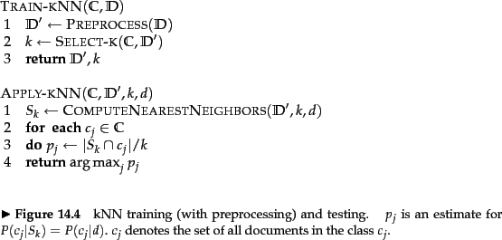
Figure 14.7 summarizes the kNN algorithm.

Worked example. The distances of the test document from the four training documents in Table 14.1 are $\vert\vec{d}_1 - \vec{d}_5 \vert =\vert\vec{d}_2 - \vec{d}_5 \vert =\vert\vec{d}_3 - \vec{d}_5 \vert \approx 1.41$ and $\vert\vec{d}_4 - \vec{d}_5 \vert =0.0$. $d_5$'s nearest neighbor is therefore $d_4$ and 1NN assigns $d_5$ to $d_4$'s class, $\overline{c}$. End worked example.