For each term ![]() , what would these
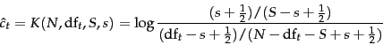
, what would these ![]() numbers look like for the whole collection? odds-ratio-ct-contingency gives a contingency table of counts of documents in the collection, where
numbers look like for the whole collection? odds-ratio-ct-contingency gives a contingency table of counts of documents in the collection, where ![]() is the number of documents that contain term
is the number of documents that contain term ![]() :
:
![\begin{example}
\begin{tabular}[t]{\vert cc\vert cc\vert c\vert}
\hline
& docum...
...\\ \hline
& Total & $S$\ & $N-S$\ & $N$\ \\ \hline
\end{tabular}
\end{example}](img727.png)
Using this, ![]() and
and
![]() and
and
Adding ![]() in this way is a simple form of
smoothing. For trials with categorical outcomes (such as
noting the presence or absence of a term),
one way to estimate the probability of
an event from data is simply to count the number of times an
event occurred divided by the total number of trials.
This is referred to as the relative frequency of the event.
Estimating the
probability as the relative frequency is the maximum
likelihood estimate (or
MLE ),
because this value
makes the observed data maximally likely. However, if we
simply use the MLE, then the probability given to events we
happened to see is usually too high, whereas other
events may be completely unseen and giving them as a
probability estimate their relative frequency of 0 is both
an underestimate, and normally breaks our models, since
anything multiplied by 0 is 0. Simultaneously decreasing
the estimated
probability of seen events and increasing the probability of
unseen events is referred to as smoothing . One
simple way of smoothing is to
add a number
in this way is a simple form of
smoothing. For trials with categorical outcomes (such as
noting the presence or absence of a term),
one way to estimate the probability of
an event from data is simply to count the number of times an
event occurred divided by the total number of trials.
This is referred to as the relative frequency of the event.
Estimating the
probability as the relative frequency is the maximum
likelihood estimate (or
MLE ),
because this value
makes the observed data maximally likely. However, if we
simply use the MLE, then the probability given to events we
happened to see is usually too high, whereas other
events may be completely unseen and giving them as a
probability estimate their relative frequency of 0 is both
an underestimate, and normally breaks our models, since
anything multiplied by 0 is 0. Simultaneously decreasing
the estimated
probability of seen events and increasing the probability of
unseen events is referred to as smoothing . One
simple way of smoothing is to
add a number ![]() to each
of the observed counts. These pseudocounts
correspond to the use of a uniform distribution over the vocabulary as a Bayesian
prior , following
Equation 59. We initially assume a uniform
distribution over events, where the size of
to each
of the observed counts. These pseudocounts
correspond to the use of a uniform distribution over the vocabulary as a Bayesian
prior , following
Equation 59. We initially assume a uniform
distribution over events, where the size of ![]() denotes
the strength of our belief in uniformity, and we then update
the probability based on observed events. Since our belief
in uniformity is weak, we use
denotes
the strength of our belief in uniformity, and we then update
the probability based on observed events. Since our belief
in uniformity is weak, we use
![]() . This
is a form of maximum a posteriori ( MAP )
estimation, where we choose the most likely point value for
probabilities based on the prior and the observed evidence,
following Equation 59. We will further discuss
methods of smoothing estimated counts to give probability
models in Section 12.2.2 (page
. This
is a form of maximum a posteriori ( MAP )
estimation, where we choose the most likely point value for
probabilities based on the prior and the observed evidence,
following Equation 59. We will further discuss
methods of smoothing estimated counts to give probability
models in Section 12.2.2 (page ![]() ); the simple method of
adding
); the simple method of
adding ![]() to each observed count will do for now.
to each observed count will do for now.