Term-document matrices and singular value decompositions

The decompositions we have been studying thus far apply to square matrices. However, the matrix we are interested in is the $\lsinoterms\times \lsinodocs$ term-document matrix $\lsimatrix$ where (barring a rare coincidence) $\lsinoterms\neq \lsinodocs$; furthermore, $\lsimatrix$ is very unlikely to be symmetric. To this end we first describe an extension of the symmetric diagonal decomposition known as the singular value decomposition . We then show in Section 18.3 how this can be used to construct an approximate version of $\lsimatrix$. It is beyond the scope of this book to develop a full treatment of the mathematics underlying singular value decompositions; following the statement of Theorem 18.2 we relate the singular value decomposition to the from Section 18.1.1 . Given $\lsimatrix$, let $U$ be the $\lsinoterms\times \lsinoterms$ matrix whose columns are the orthogonal eigenvectors of $\lsimatrix\lsimatrix^T$, and $V$ be the $\lsinodocs\times \lsinodocs$ matrix whose columns are the orthogonal eigenvectors of $\lsimatrix^T\lsimatrix$. Denote by $\lsimatrix^T$ the transpose of a matrix $\lsimatrix$.

Theorem. Let $r$ be the rank of the $\lsinoterms\times \lsinodocs$ matrix $\lsimatrix$. Then, there is a singular-value decomposition ( SVD for short) of $\lsimatrix$ of the form

$$\lsimatrix=U\Sigma V^T,$$ (232)

where

1. The eigenvalues $\lambda_1,\ldots , \lambda_r$ of $\lsimatrix\lsimatrix^T$ are the same as the eigenvalues of $\lsimatrix^T\lsimatrix$;
2. For $1\leq i\leq r$, let $\sigma_i=\sqrt{\lambda_i}$, with $\lambda_i\geq \lambda_{i+1}$. Then the $\lsinoterms\times \lsinodocs$ matrix $\Sigma$ is composed by setting $\Sigma_{ii}=\sigma_i$ for $1\leq i\leq r$, and zero otherwise.

End theorem.

The values $\sigma_i$ are referred to as the singular values of $\lsimatrix$. It is instructive to examine the relationship of Theorem 18.2 to Theorem 18.1.1; we do this rather than derive the general proof of Theorem 18.2, which is beyond the scope of this book.

By multiplying Equation 232 by its transposed version, we have

$$\lsimatrix\lsimatrix^T=U\Sigma V^T \; V\Sigma U^T = U\Sigma^2 U^T.$$ (233)

Note now that in Equation 233, the left-hand side is a square symmetric matrix real-valued matrix, and the right-hand side represents its symmetric diagonal decomposition as in Theorem 18.1.1. What does the left-hand side $\lsimatrix\lsimatrix^T$ represent? It is a square matrix with a row and a column corresponding to each of the $\lsinoterms$ terms. The entry $(i,j)$ in the matrix is a measure of the overlap between the $i$th and $j$th terms, based on their co-occurrence in documents. The precise mathematical meaning depends on the manner in which $\lsimatrix$ is constructed based on term weighting. Consider the case where $\lsimatrix$ is the term-document incidence matrix of page 1.1 , illustrated in Figure 1.1 . Then the entry $(i,j)$ in $\lsimatrix\lsimatrix^T$ is the number of documents in which both term $i$ and term $j$ occur.

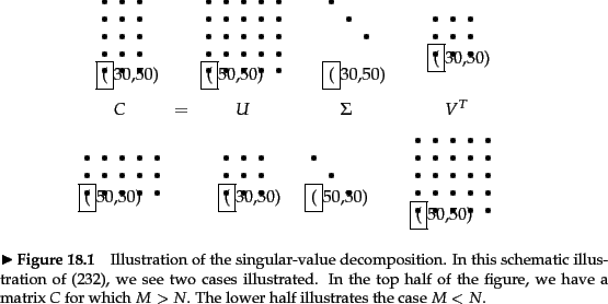
When writing down the numerical values of the SVD, it is conventional to represent $\Sigma$ as an $r\times r$ matrix with the singular values on the diagonals, since all its entries outside this sub-matrix are zeros. Accordingly, it is conventional to omit the rightmost $M-r$ columns of $U$ corresponding to these omitted rows of $\Sigma$; likewise the rightmost $N-r$ columns of $V$ are omitted since they correspond in $V^T$ to the rows that will be multiplied by the $N-r$ columns of zeros in $\Sigma$. This written form of the SVD is sometimes known as the reduced SVD or truncated SVD and we will encounter it again in Exercise 18.3 . Henceforth, our numerical examples and exercises will use this reduced form.

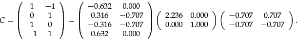
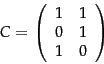
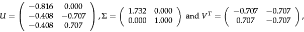
Worked example. We now illustrate the singular-value decomposition of a $4\times 2$ matrix of rank 2; the singular values are $\Sigma_{11}=2.236$ and $\Sigma_{22}=1$.

$$\lsimatrix=\left( \begin{array}{cc} 1 & -1 \\ 0 & 1 \\ ... ... -0.707 & 0.707\\ -0.707 & -0.707 \\ \end{array} \right).$$ (234)

End worked example.

As with the matrix decompositions defined in Section 18.1.1 , the singular value decomposition of a matrix can be computed by a variety of algorithms, many of which have been publicly available software implementations; pointers to these are given in Section 18.5 .

Exercises.

• Let
  

  $$\lsimatrix=\left( \begin{array}{cc} 1 & 1 \\ 0 & 1 \\ 1 & 0 \\ \end{array} \right)$$ (235)

  
  
  be the term-document incidence matrix for a collection. Compute the co-occurrence matrix $\lsimatrix\lsimatrix^T$. What is the interpretation of the diagonal entries of $\lsimatrix\lsimatrix^T$ when $\lsimatrix$ is a term-document incidence matrix?

• Verify that the SVD of the matrix in Equation 235 is
  

  $$U=\left( \begin{array}{cc} -0.816 & 0.000 \\ -0.408 & -... ... -0.707 & -0.707 \\ 0.707 & -0.707\\ \end{array} \right),$$ (236)

  
  
  by verifying all of the properties in the statement of Theorem 18.2.

• Suppose that $\lsimatrix$ is a binary term-document incidence matrix. What do the entries of $\lsimatrix^T\lsimatrix$ represent?

• Let
  

  $$\lsimatrix=\left( \begin{array}{ccc} 0 & 2 & 1 \\ 0 & 3 & 0 \\ 2 & 1 & 0 \\ \end{array} \right)$$ (237)

  
  
  be a term-document matrix whose entries are term frequencies; thus term 1 occurs 2 times in document 2 and once in document 3. Compute $\lsimatrix\lsimatrix^T$; observe that its entries are largest where two terms have their most frequent occurrences together in the same document.