Time complexity of HAC

The complexity of the naive HAC algorithm in Figure 17.2 is $\Theta(N^3)$ because we exhaustively scan the $N \times N$ matrix

for the largest similarity in each of

iterations.

$\begin{figure} % latex2html id marker 26593 \begin{algorithm}{EfficientHAC}{\vec... ...a made up example showing $P[5]$\ for a $5 \times 5$\ matrix $C$. } \end{figure}$

For the four HAC methods discussed in this chapter a more efficient algorithm is the priority-queue algorithm shown in Figure 17.8 . Its time complexity is $\Theta(N^2 \log N)$ . The rows

of the $N \times N$ similarity matrix

are sorted in decreasing order of similarity in the priority queues

. $P[k].\mbox{\sc max()}$ then returns the cluster in

that currently has the highest similarity with $\omega_k$ , where we use $\omega_k$ to denote the $k^{th}$ cluster as in Chapter 16 . After creating the merged cluster of $\omega_{k_1}$ and $\omega_{k_2}$ , $\omega_{k_1}$ is used as its representative. The function SIM computes the similarity function for potential merge pairs: largest similarity for single-link, smallest similarity for complete-link, average similarity for GAAC (Section 17.3 ), and centroid similarity for centroid clustering (Section 17.4 ). We give an example of how a row of

is processed (Figure 17.8 , bottom panel). The loop in lines 1-7 is $\Theta(N^2)$ and the loop in lines 9-21 is $\Theta(N^2 \log N)$ for an implementation of priority queues that supports deletion and insertion in $\Theta(\log N)$ . The overall complexity of the algorithm is therefore $\Theta(N^2 \log N)$ . In the definition of the function SIM, $\vec{v}_m$ and $\vec{v}_\oldell$ are the vector sums of $\omega_{k_1} \cup \omega_{k_2}$ and $\omega_\oldell$ , respectively, and

and $N_\oldell$ are the number of documents in $\omega_{k_1} \cup \omega_{k_2}$ and $\omega_\oldell$ , respectively.

The argument of EFFICIENTHAC in Figure 17.8 is a set of vectors (as opposed to a set of generic documents) because GAAC and centroid clustering ( and 17.4 ) require vectors as input. The complete-link version of EFFICIENTHAC can also be applied to documents that are not represented as vectors.

$\begin{figure} % latex2html id marker 26700 \begin{algorithm}{SingleLinkClusteri... ...y $I[i]$\ and will therefore be ignored when updating $NBM[i_1]$. } \end{figure}$

For single-link, we can introduce a next-best-merge array (NBM) as a further optimization as shown in Figure 17.9 . NBM keeps track of what the best merge is for each cluster. Each of the two top level for-loops in Figure 17.9 are $\Theta(N^2)$ , thus the overall complexity of single-link clustering is $\Theta(N^2)$ .

Can we also speed up the other three HAC algorithms with an NBM array? We cannot because only single-link clustering is best-merge persistent . Suppose that the best merge cluster for $\omega_k$ is $\omega_j$ in single-link clustering. Then after merging $\omega_j$ with a third cluster $\omega_i \neq \omega_k$ , the merge of $\omega_i$ and $\omega_j$ will be $\omega_k$ 's best merge cluster (Exercise 17.10 ). In other words, the best-merge candidate for the merged cluster is one of the two best-merge candidates of its components in single-link clustering. This means that

can be updated in $\Theta(N)$ in each iteration - by taking a simple max of two values on line 14 in Figure 17.9 for each of the remaining $\leq N$ clusters.

$\begin{figure} % latex2html id marker 26751 \par \psset{unit=0.5cm} \par \begin{... ...ke single-link, $d_3$'s best-merge cluster would be $\{d_1,d_2\}$.} \end{figure}$

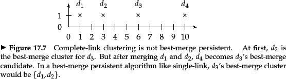
Figure 17.10 demonstrates that best-merge persistence does not hold for complete-link clustering, which means that we cannot use an NBM array to speed up clustering. After merging

's best merge candidate

with cluster

, an unrelated cluster

becomes the best merge candidate for

. This is because the complete-link merge criterion is non-local and can be affected by points at a great distance from the area where two merge candidates meet.

In practice, the efficiency penalty of the $\Theta(N^2 \log N)$ algorithm is small compared with the $\Theta(N^2)$ single-link algorithm since computing the similarity between two documents (e.g., as a dot product) is an order of magnitude slower than comparing two scalars in sorting. All four HAC algorithms in this chapter are $\Theta(N^2)$ with respect to similarity computations. So the difference in complexity is rarely a concern in practice when choosing one of the algorithms.