


Next: An appraisal and some
Up: The Binary Independence Model
Previous: Probability estimates in practice
Contents
Index
Probabilistic approaches to relevance feedback
We can use (pseudo-)relevance feedback, perhaps in an iterative process of estimation, to get a more accurate estimate of  .
The probabilistic approach to relevance feedback works as follows:
.
The probabilistic approach to relevance feedback works as follows:
- Guess initial estimates of and
 . This
can be done using the probability estimates of the previous
section. For instance, we can assume that is constant over all
. This
can be done using the probability estimates of the previous
section. For instance, we can assume that is constant over all  in the query, in particular, perhaps taking
 .
.
- Use the current estimates of and to determine a best guess at the set of relevant documents
 . Use this model
to retrieve a set of candidate relevant documents, which we present to the user.
. Use this model
to retrieve a set of candidate relevant documents, which we present to the user.
- We interact with the user to refine the model of
 . We do this by learning from the user relevance judgments for some subset of documents
  .
Based on relevance judgments, is partitioned into two subsets:
.
Based on relevance judgments, is partitioned into two subsets:
 and
and
 , which is disjoint from .
- We reestimate and on the basis of known relevant and nonrelevant documents. If the sets
 and
and  are large enough, we may be able to estimate these quantities directly from these documents as maximum likelihood estimates:
 |
(77) |
(where  is the set of documents in containing ). In practice, we usually need to smooth these estimates. We can do this by adding
  to both the count
  and to the number of relevant documents not containing the term, giving:
 |
(78) |
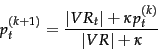
However, the set of documents judged by the user () is usually very small, and so the resulting statistical estimate is quite unreliable (noisy), even if the estimate is smoothed. So it is often better to combine the new information with the original guess in a process of Bayesian updating . In this case we have:
 |
(79) |
Here  is the
  estimate for in an
iterative updating process and is used as a Bayesian prior in the next iteration with a weighting of
estimate for in an
iterative updating process and is used as a Bayesian prior in the next iteration with a weighting of  . Relating this equation back to Equation 59 requires a bit more probability theory than we have presented here (we need to use a beta distribution prior, conjugate to the Bernoulli random variable
  ). But the form of the resulting equation is quite straightforward: rather than uniformly distributing pseudocounts, we now distribute a total of pseudocounts according to the previous estimate, which acts as the prior distribution.
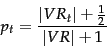
In the absence of other evidence (and assuming that the user is perhaps indicating roughly 5 relevant or nonrelevant documents) then a value of around
). But the form of the resulting equation is quite straightforward: rather than uniformly distributing pseudocounts, we now distribute a total of pseudocounts according to the previous estimate, which acts as the prior distribution.
In the absence of other evidence (and assuming that the user is perhaps indicating roughly 5 relevant or nonrelevant documents) then a value of around  is perhaps appropriate. That is, the prior is strongly weighted so that the estimate does not change too much from the evidence provided by a very small number of documents.
- Repeat the above process from step 2, generating a succession of approximations to and hence , until the user is satisfied.
It is also straightforward to derive a pseudo-relevance feedback version of this algorithm, where we simply pretend that  . More briefly:
- Assume initial estimates for and as above.
- Determine a guess for the size of the relevant document set. If unsure, a conservative (too small) guess is likely to be best. This motivates use of a fixed size set of highest ranked documents.
- Improve our guesses for and . We choose from the methods of and 79 for re-estimating , except now based on the set instead of . If we let
 be the subset of documents in containing and use add smoothing , we get:
 |
(80) |
and if we assume that documents that are not retrieved are nonrelevant then we can update our estimates as:
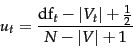 |
(81) |
- Go to step 2 until the ranking of the returned results converges.
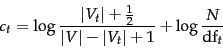
Once we have a real estimate for then the  weights used in the
  value look almost like a tf-idf value. For instance, using Equation 73, Equation 76, and Equation 80, we have:
![\begin{displaymath}
c_t = \log \left[\frac{p_t}{1-p_t}\cdot\frac{1-u_t}{u_t}\rig...
...vert V\vert - \vert V_t\vert + 1}\cdot\frac{N}{\docf_t}\right]
\end{displaymath}](img761.png) |
(82) |
But things aren't quite the same:  measures the (estimated) proportion of relevant documents that the term
  occurs in, not term frequency. Moreover, if we apply log identities:
 |
(83) |
we see that we are now adding the two log scaled components rather than multiplying them.
Exercises.
Next: An appraisal and some
Up: The Binary Independence Model
Previous: Probability estimates in practice
Contents
Index
© 2008 Cambridge University Press
This is an automatically generated page. In case of formatting errors you may want to look at the PDF edition of the book.
2009-04-07