Next: Assessing as a feature
Up: Feature selection
Previous: Mutual information
Contents
Index
Another popular feature selection
method is  .
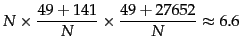
In statistics, the test is
applied to test the independence of two events,
where two events A and B are defined to be
independent if
.
In statistics, the test is
applied to test the independence of two events,
where two events A and B are defined to be
independent if
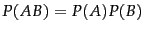 or, equivalently,
 and
and
 . In
feature selection, the two events are occurrence of the
term and occurrence of the class.
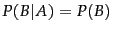
We then rank terms with respect to the following
quantity:
. In
feature selection, the two events are occurrence of the
term and occurrence of the class.
We then rank terms with respect to the following
quantity:
 |
|
|
(133) |
where  and
and  are defined as in Equation 130.
  is the observed frequency in
 and
and  the
expected frequency. For example,
the
expected frequency. For example,  is the
expected frequency of
is the
expected frequency of  and
and  occurring together
in a document assuming that term and class are independent.
occurring together
in a document assuming that term and class are independent.
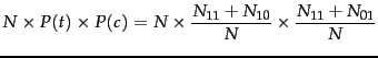
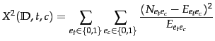
Worked example. We first
compute for the
data in Example 13.5.1:
where  is the total number of documents as before.
We compute the other
 in the same way:
Plugging these values into
Equation 133, we get a  value of 284:
 |
|
|
(136) |
End worked example.
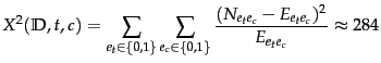
is a measure of how much expected counts and observed
counts deviate from each other. A high value of
indicates that the hypothesis of independence, which implies
that expected and observed counts are similar, is
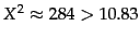
incorrect. In our example,
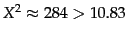 . Based
on Table 13.6 , we can reject the hypothesis that
poultry and export are independent with only
a 0.001 chance of being wrong.
. Based
on Table 13.6 , we can reject the hypothesis that
poultry and export are independent with only
a 0.001 chance of being wrong.![[*]](http://nlp.stanford.edu/IR-book/html/icons/footnote.png) Equivalently, we say that the outcome
Equivalently, we say that the outcome
 is statistically
significant at the 0.001 level. If the two events are
dependent, then the occurrence of the term makes the occurrence
of the class more likely (or less likely), so it should be
helpful as a feature. This is the rationale of
feature selection.
is statistically
significant at the 0.001 level. If the two events are
dependent, then the occurrence of the term makes the occurrence
of the class more likely (or less likely), so it should be
helpful as a feature. This is the rationale of
feature selection.
Table 13.6:
Critical values of the
distribution with one degree of freedom. For example, if
the two events are
independent, then
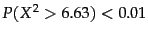 . So for
 the assumption of independence can be rejected with 99% confidence.
| |  |
critical value |
|
| | 0.1 |
2.71 |
|
| | 0.05 |
3.84 |
|
| | 0.01 |
6.63 |
|
| | 0.005 |
7.88 |
|
| | 0.001 |
10.83 |
|
An arithmetically simpler way of computing
 is the
following:
is the
following:
 |
(137) |
This is equivalent to Equation 133
(Exercise 13.6 ).
Subsections
Next: Assessing as a feature
Up: Feature selection
Previous: Mutual information
Contents
Index
© 2008 Cambridge University Press
This is an automatically generated page. In case of formatting errors you may want to look at the PDF edition of the book.
2009-04-07