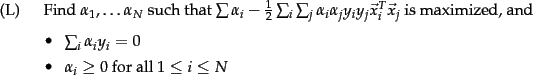
For two-class, separable training data sets, such as the one in
Figure 14.8 (page ![]() ), there are lots of
possible linear separators. Intuitively, a decision boundary
drawn in the middle of
the void between data items of the two classes seems better
than one which approaches very close to examples of one or both classes.
While some learning methods such as the
perceptron algorithm (see references in vclassfurther)
find just any linear separator, others, like Naive Bayes, search for
the best linear separator according to some criterion. The SVM in
particular defines the criterion to be looking for a decision surface that is
maximally far away from any data point. This distance from the
decision surface to the closest data point determines the
margin of the classifier.
This method of construction necessarily means
that the decision function for an SVM is fully specified by a (usually
small) subset of the data which defines the position of the separator.
These points are referred to as the support
vectors (in a vector space, a point can be thought of as a vector
between the origin and that point). Figure 15.1 shows the margin and support
vectors for a sample problem. Other data points play no part in
determining the decision surface that is chosen.
), there are lots of
possible linear separators. Intuitively, a decision boundary
drawn in the middle of
the void between data items of the two classes seems better
than one which approaches very close to examples of one or both classes.
While some learning methods such as the
perceptron algorithm (see references in vclassfurther)
find just any linear separator, others, like Naive Bayes, search for
the best linear separator according to some criterion. The SVM in
particular defines the criterion to be looking for a decision surface that is
maximally far away from any data point. This distance from the
decision surface to the closest data point determines the
margin of the classifier.
This method of construction necessarily means
that the decision function for an SVM is fully specified by a (usually
small) subset of the data which defines the position of the separator.
These points are referred to as the support
vectors (in a vector space, a point can be thought of as a vector
between the origin and that point). Figure 15.1 shows the margin and support
vectors for a sample problem. Other data points play no part in
determining the decision surface that is chosen.
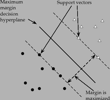
![\includegraphics[width=4.5in]{band-aids.eps}](img1261.png) An intuition for large-margin classification.Insisting on a
large margin reduces the capacity of the model: the range of angles
at which the fat decision surface can be placed is smaller than for a
decision hyperplane (cf. vclassline).
An intuition for large-margin classification.Insisting on a
large margin reduces the capacity of the model: the range of angles
at which the fat decision surface can be placed is smaller than for a
decision hyperplane (cf. vclassline).
Maximizing the margin seems good because points near the decision surface represent very uncertain classification decisions: there is almost a 50% chance of the classifier deciding either way. A classifier with a large margin makes no low certainty classification decisions. This gives you a classification safety margin: a slight error in measurement or a slight document variation will not cause a misclassification. Another intuition motivating SVMs is shown in Figure 15.2 . By construction, an SVM classifier insists on a large margin around the decision boundary. Compared to a decision hyperplane, if you have to place a fat separator between classes, you have fewer choices of where it can be put. As a result of this, the memory capacity of the model has been decreased, and hence we expect that its ability to correctly generalize to test data is increased (cf. the discussion of the bias-variance tradeoff in Chapter 14 , page 14.6 ).
Let us formalize an SVM with algebra. A decision hyperplane
(page 14.4 ) can be
defined by an intercept term ![]() and a decision hyperplane normal vector
and a decision hyperplane normal vector
![]() which is
perpendicular to the hyperplane. This vector is commonly referred to
in the machine learning literature as the weight vector .
To choose among
all the hyperplanes that are perpendicular to the normal vector, we
specify the intercept term
which is
perpendicular to the hyperplane. This vector is commonly referred to
in the machine learning literature as the weight vector .
To choose among
all the hyperplanes that are perpendicular to the normal vector, we
specify the intercept term ![]() .
Because the hyperplane is perpendicular to the normal vector, all
points
.
Because the hyperplane is perpendicular to the normal vector, all
points ![]() on the hyperplane satisfy
on the hyperplane satisfy
![]() .
Now suppose that we have a set of
training data points
.
Now suppose that we have a set of
training data points
![]() , where each member is a pair of a point
, where each member is a pair of a point ![]() and a class label
and a class label ![]() corresponding to it.
corresponding to it.![]() For SVMs, the two data classes are always named
For SVMs, the two data classes are always named ![]() and
and ![]() (rather than 1 and 0), and the intercept term is always
explicitly represented as
(rather than 1 and 0), and the intercept term is always
explicitly represented as ![]() (rather than being folded into the weight
vector
(rather than being folded into the weight
vector ![]() by adding an extra always-on feature). The
math works out much more cleanly if you do things this way, as we
will see almost immediately in the definition of functional margin. The
linear classifier is then:
by adding an extra always-on feature). The
math works out much more cleanly if you do things this way, as we
will see almost immediately in the definition of functional margin. The
linear classifier is then:
We are confident in the classification of a point if it is far away from
the decision boundary. For a given data set and decision hyperplane, we
define the functional margin of the
![]() example
example ![]() with respect to a hyperplane
with respect to a hyperplane
![]() as the quantity
as the quantity
![]() . The
functional margin of a data set with respect to a decision surface is then twice the
functional margin of any of the points in the data set with minimal functional
margin (the factor of 2 comes from measuring across
the whole width of the margin, as in Figure 15.3 ).
However, there is a problem with using this
definition as is: the value is underconstrained, because
we can always make the functional margin as big as we wish
by simply scaling up
. The
functional margin of a data set with respect to a decision surface is then twice the
functional margin of any of the points in the data set with minimal functional
margin (the factor of 2 comes from measuring across
the whole width of the margin, as in Figure 15.3 ).
However, there is a problem with using this
definition as is: the value is underconstrained, because
we can always make the functional margin as big as we wish
by simply scaling up ![]() and
and ![]() . For example, if we replace
. For example, if we replace ![]() by
by ![]() and
and ![]() by
by ![]() then the functional margin
then the functional margin
![]() is five times as large. This suggests that we need to place
some constraint on the size of the
is five times as large. This suggests that we need to place
some constraint on the size of the ![]() vector. To get a sense of
how to do that, let us look at the actual geometry.
vector. To get a sense of
how to do that, let us look at the actual geometry.
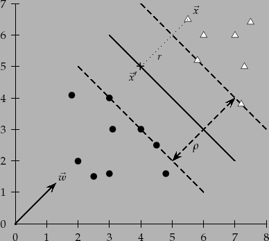
What is the Euclidean distance from a point ![]() to the decision
boundary? In Figure 15.3 , we denote by
to the decision
boundary? In Figure 15.3 , we denote by ![]() this distance.
We know that the shortest distance between a point and a
hyperplane is perpendicular to the plane, and hence, parallel to
this distance.
We know that the shortest distance between a point and a
hyperplane is perpendicular to the plane, and hence, parallel to
![]() . A unit vector in this direction is
. A unit vector in this direction is
![]() .
The dotted line in the diagram is then a translation of the vector
.
The dotted line in the diagram is then a translation of the vector
![]() .
Let us label the point on the hyperplane closest to
.
Let us label the point on the hyperplane closest to ![]() as
as
![]() . Then:
. Then:
| (166) |
| (167) |
Since we can scale the functional margin as we please, for convenience
in solving large SVMs, let us choose to require
that the functional margin of
all data points is at least 1 and that it is equal to 1 for at least
one data vector. That is, for all items in the data:
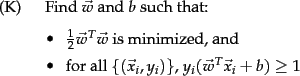
We are now optimizing a quadratic function subject to linear constraints. Quadratic optimization problems are a standard, well-known class of mathematical optimization problems, and many algorithms exist for solving them. We could in principle build our SVM using standard quadratic programming (QP) libraries, but there has been much recent research in this area aiming to exploit the structure of the kind of QP that emerges from an SVM. As a result, there are more intricate but much faster and more scalable libraries available especially for building SVMs, which almost everyone uses to build models. We will not present the details of such algorithms here.
However, it will be helpful to what follows to understand the shape of
the solution of such an optimization problem.
The solution involves constructing a dual problem where a
Lagrange multiplier ![]() is associated with each constraint
is associated with each constraint
![]() in the
primal problem:
in the
primal problem:
The solution is then of the form:
![]()
In the solution, most of the ![]() are zero. Each non-zero
are zero. Each non-zero
![]() indicates that the corresponding
indicates that the corresponding ![]() is a support vector.
The classification function is then:
is a support vector.
The classification function is then:
To recap, we start with a training data set. The data set
uniquely defines the best separating hyperplane, and we feed
the data through a quadratic optimization procedure to find
this plane. Given a new point ![]() to classify, the
classification function
to classify, the
classification function ![]() in either
Equation 165 or Equation 170 is
computing the projection of the point onto the hyperplane
normal. The sign of this function determines the
class to assign to the point. If the point is within
the margin of the classifier (or another confidence
threshold
in either
Equation 165 or Equation 170 is
computing the projection of the point onto the hyperplane
normal. The sign of this function determines the
class to assign to the point. If the point is within
the margin of the classifier (or another confidence
threshold ![]() that we might have determined to minimize
classification mistakes) then the classifier can return
``don't know'' rather than one of the two classes. The
value of
that we might have determined to minimize
classification mistakes) then the classifier can return
``don't know'' rather than one of the two classes. The
value of ![]() may also be transformed into a
probability of classification; fitting a sigmoid to
transform the values is standard
(Platt, 2000). Also, since the
margin is constant, if the model includes dimensions from various
sources, careful rescaling of some dimensions may be
required. However, this is not a problem if our documents (points) are
on the unit hypersphere.
may also be transformed into a
probability of classification; fitting a sigmoid to
transform the values is standard
(Platt, 2000). Also, since the
margin is constant, if the model includes dimensions from various
sources, careful rescaling of some dimensions may be
required. However, this is not a problem if our documents (points) are
on the unit hypersphere.
Worked example. Consider building an SVM over the (very little) data set shown in
Figure 15.4 . Working geometrically, for an example like this,
the maximum margin weight
vector will be parallel to the shortest line connecting points of the two
classes, that is, the line between ![]() and
and ![]() , giving a
weight vector of
, giving a
weight vector of ![]() .
The optimal decision surface is orthogonal to that line and intersects
it at the halfway point. Therefore, it passes through
.
The optimal decision surface is orthogonal to that line and intersects
it at the halfway point. Therefore, it passes through ![]() . So,
the SVM decision boundary is:
. So,
the SVM decision boundary is:
| (171) |
Working algebraically, with the standard constraint that
![]() , we seek
to minimize
, we seek
to minimize
![]() . This happens when this constraint is satisfied with
equality by the two support vectors. Further we know that the
solution is
. This happens when this constraint is satisfied with
equality by the two support vectors. Further we know that the
solution is
![]() for some
for some ![]() . So we have that:
. So we have that:
The margin ![]() is
is
![]() . This answer can be confirmed geometrically by examining Figure 15.4 .
. This answer can be confirmed geometrically by examining Figure 15.4 .
End worked example.
Exercises.
The training command for SVMlight is then:1 1:2 2:3
1 1:2 2:0
svm_learn -c 1 -a alphas.dat train.dat model.datThe -c 1 option is needed to turn off use of the slack variables that we discuss in Section 15.2.1 . Check that the norm of the weight vector agrees with what we found in small-svm-eg. Examine the file alphas.dat which contains the

\end{pspicture}\par
\end{figure}](img1299.png)